Drying and Storage Engineering

Lesson 9. Modeling And Simulation Of Drying Process

9.1 Macroscopic approach

The macroscopic approach assumes the tissue is homogeneous and the modelling is carried out on the lumped properties of cell wall, cell membrane and cell vacuole (Yao and Le Maguer, 1996; Azuara et al., 1992). The models available in literature can be classified under the following approaches:

1. Estimation of diffusion coefficients for water loss and solid gain by using Fick’s second law of diffusion.

2. Estimation of water loss and solid gain as a function of time, temperature and initial concentration of the medium (Empirical models).

3. Based on cellular structure according to non-reversible thermodynamic principles.

4. Prediction of equilibrium moisture loss.

5. Pressure gradient dependent modeling accounting the capillary and external pressure effects (Hydrodynamic mechanism).

6. Artificial Neural Network (ANN) modeling

7. Statistical modeling like stochastic approach, Weibull probabilistic distribution and multiple regression.

9.2 Microscopic approach

The microscopic approach recognizes the heterogeneous properties of the tissue and the complex cellular structure is represented by a simplified conceptual model. The modeling of the cellular structural is attempted by very few researchers.

9.3 Modeling and simulation of temperature and moisture distribution in foods during drying

Table 9.3 Mathematical models used to test the drying kinetics

Model Name	Model	Reference
Newton	MR = exp(-kt)	Liu and Bakker-Arkema(1997), Nellist (1987)
Page	MR = exp(-ktn)	Agrawal and Singh (1977), Bruce (1985)
Henderson and  Pebis	MR = a exp(-kt)	Pal and Chakraverty (1997), Rahman and Perera (1996)
Two-Term	MR = a exp(bt) + c exp(dt)	Henderson (1974)
Asymptotic Logarithmic	MR = a exp(-kt)+b	Yaldız and Ertekin (2001)
Wang and Singh	MR =1+at+bt2	Wang and Singh (1978)
Diffusion approximation	MR = a exp(-kt)+(1-a) exp(-kat)	Yaldız and Ertekin (2001)
Two term Exponential	MR = a exp(-kt) + (1-a) exp(-kat)	Wang and Singh (1978)
Verma et. al.	MR = a exp(-kx)+(1-a) exp(-gt)	Verma et. al (1985)
Modified Henderson and Pabis	MR = a exp(-kx)+b exp(-gx)           +c exp(-gx)	Karathanos and Belessiotis (1999)

The non-uniformity in temperature and moisture distributions is the main reason for unacceptable food quality of microwaved products. Some of the key factors that influence the uniformity of temperature distribution are the dielectric and thermo-physical properties of the product, frequency and power of the incident microwave energy, and the geometry and dimensions of the product (Jun and Puri, 2004). The successful design of industrial microwave application can be done with the aid of modeling techniques which relate electrical and physical properties of foods (Van Remmen et al., 1996). The literature shows the two approaches of modeling of power deposition patterns: (1) making use of Maxwell’s equations for electromagnetic field, and (2) using Lambert’s law in which power is attenuated exponentially as a function of distance of one dimensional penetration into the material. However, the Lambert’s law can be used for samples thicker than about three times the characteristics penetration depth of microwaves, but the law fails for thinner samples. It turns out that Lambert’s law is inapplicable for most foods prepared in home microwave ovens. Therefore, Maxwell’s equation must be used to accurately describe the propagation and absorption of radiation (Ayappa et al., 1991). Generally, finite difference, finite element and boundary element methods are used to solve the Maxwell’s equations to obtain power deposition patterns in slabs, cylinders and spheres (Van Remmen et al., 1996).

Finite difference approximations have been used to obtain reasonable estimation of internal temperature and moisture profiles during microwave heating. However, most of these models were for microwave-convective heating. Very few literatures focus on modeling of microwave-vacuum drying of sliced and individual food particles. Lian et al. (1997) described the coupled heat and moisture transfer during microwave vacuum drying of a soluble food concentrate. They considered the moisture transfer as a combination of simultaneous water (liquid) and vapour transfer. Pandit and Prasad (2003) have developed simplified heat and mass transfer model to predict moisture and temperature changes during microwave drying of various shaped food materials. Kiranoudis et al. (1997) studied the mathematical model of the microwave vacuum drying kinetics of some fruits. An empirical mass transfer model, involving a basic parameter of phenomenological nature, was used and the influence of process variables was examined by embodying them to the drying constant.

9.4 Mass transfer kinetics during osmotic dehydration

The osmotic dehydration process different than other drying processes as mass transfer takes place in liquid form (water comes out of product without phase change). Therefore, different models are available for the process. During osmotic dehydration, two resistances oppose mass transfer, one internal and the other external. The fluid dynamics of the solid fluid interface governs the external resistance whereas, the much more complex internal resistance is influenced by cell tissue structure, cellular membrane permeability, deformation of vegetable/fruit pieces and the interaction between the different mass fluxes. Under the usual treatment conditions, the external resistance is negligible compared to the internal one. Variability in biological product characteristics produces major difficulties regarding process modeling and optimization. Mass transfer is affected by variety, maturity level and composition of product. The complex non-homogenous structure of natural tissues complicates any effort to study and understand the mass transport mechanisms of several interacting counter current flows (water, osmotic solute, soluble product solids).

A mathematical model developed by Azuara et al. (1992) was used to study the mass transfer in osmotic dehydration of carrot slices. The various parameters considered for the model were moisture loss at any time (ML_t), moisture loss at equilibrium ( ), solid gained at any time (SG_t), solids gained at equilibrium ( ) and the time of osmotic dehydration (t). The models are as follows:

The plots of t/ML_­t  vs. t and t/SG_t  vs. t would be linear, the parameters could be determined from the intercept and slope. The Eqns. 3.1 and 3.3 could then be used to predict the mass transfer kinetics. S₁ and S₂ are the constants related to the rates of water and solid diffusion, respectively. The terms indicate that 1/S1 or 1/S2 represent the time required for half of the diffusible matter (water or solids) to diffuse out or enter in the product, respectively. Further, as the time t becomes much longer (that is, t ® ¥) than the values of that 1/S1 or 1/S2, the water loss or the solid gain, ML_t or SG_t, approaches equilibrium value, ML_¥ or SG_¥, asymptotically.

In above equations, the values of parameters S₁, ML_¥, S₂ and SG_¥ can be estimated from short duration osmotic kinetic data by performing linear regression or graphical plotting of the above equations in the linearized form.

9.5 Mathematical Modeling of Heat and Mass Transfer in Product by Microwave Assisted Drying

For proper equipment design, process optimization and improvement of final product quality, accurate prediction of the heat and moisture transfer in the product is vital. Many researchers have modeled the heat and moisture transfer in the food products during microwave heating and drying. They used numerical techniques based on the finite difference method, finite element method and transmission line matrix method to simulate the microwave heating with varying degree of accuracy.

9.6 Heat transfer and temperature profile within the product

In microwave heating, the governing energy balance equation includes a heat generation term Q by dielectric heating. Temperature changes at any location within a food during microwave drying are affected by thermal diffusion, generation of heat by microwaves and evaporation of moisture. Mathematically, it is represented as:

 

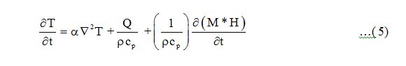
where, T is the product temperature, t is the time, Q is the conversion of microwave energy to heat per unit volume, M is the moisture concentration and H is enthalpy of moisture. The parameters  a, r and c_p are the thermal diffusivity, density and specific heat of the material, respectively.

The heat generated per unit volume of material (Q) is the conversion of electromagnetic energy in to heat energy. Its relationship with the average electric field intensity (E_rms) at that location can be derived from Maxwell’s equations of electromagnetic waves as shown by Metaxax and Meredith (1983):

 

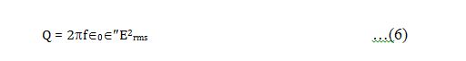
where, f  is the frequency of microwaves, Î₀  is the dielectric constant of free space and β is the loss factor of food being heated. At a given frequency, the dielectric loss factor is a function of the composition of food materials and its temperature.

9.7 Mass transfer and moisture profiles

Assuming the food material as a capillary porous body, the governing equation for the internal moisture transport process can be written as:

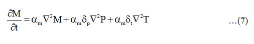
where, M is the total moisture content (liquid and vapour phase); a_m is the moisture diffusivity; d_p and d_t are the pressure and thermal gradient coefficients, respectively. The three terms in the right hand side of Eqn. 3.17 represent moisture movement due to concentration, pressure and temperature gradients, respectively. Flow due to thermal gradient is generally ignored during microwave drying of solid moist foods and the moisture movement is considered due to the pressure and concentration gradients.

9.8 Boundary and initial conditions

The generalized boundary conditions for microwave heating can be written as:

 

where, ‘x’ represents the direction normal to the boundary and ‘k_t’ is the thermal conductivity of the food material. The first term of the right hand side is for convective heat transfer at the surface with ‘h’, the convective heat transfer coefficient and ‘T_¥’, the air temperature. Convective heat loss for a food under vacuum would be much lower due to low temperature gradient. The second term of the above equation involves radiative heat loss by the food material and T_s is the temperature of the surface facing the food material. The quantities Î and s are the surface emissivity and Stefan-Boltzman constant, respectively. Radiative heat transfer is important when the surfaces of the material act as susceptors. Evaporation (m_w) at the surface is more important in microwave heating than in conventional heating because more moisture moves from the interior (Datta, 1990).

The boundary conditions for food samples in drying are featured by convective cooling and surface moisture loss. That is:

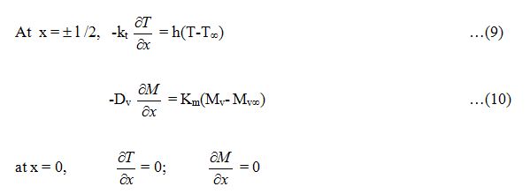
The initial sample temperature and moisture content are considered to be uniform

i.e. T = T₀;       M_v = M_v0;                           M = M₀

where, l is the thickness of slices, M_v0 is the saturated vapour concentration at T₀ and M₀ is the initial moisture concentration of the food material.