Food Processing Plant Design & Layout

Lesson 14: Plant operation

In setting up operations and designing material handling systems, it is essential that an analysis be made of the entire plant product flow. This analysis show the raw product in, the major product movement, the specialized or branch movements, the processes, the storages for the various products, and the out movements. It is particularly important to note the areas where high density traffic is found. It is also important to note the sequence of movements and provide for them so that the whole operation will move forward smoothly. The designer should take advantage of the many new material handling methods and equipment, utilizing each one where it is crates, cans, etc. can be moved by means of chain conveyors or they may be moved by trucks or pallets. Surprisingly enough, there may be places where some handling can best be made by means of manual labour.

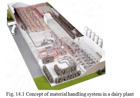
Material handling systems for food products should be carefully selected so that it will not be affected by temperature change or severe vibrations. The material handling system should be simple in design, having ease of lubrication, corrosion resistant and low maintenance. The use of automatic stopping and starting controls, speed regulators, switches, and over-load safety devices are all important. Fig. 14.1 shows concept of material handling system in a dairy plant.

 

Research in operations or operation research provide solution for above said complex problems arising in the direction and management of large systems of men, machines, materials and money in industry and business governance.

The significant features of operations research can be stated as:

• Decision making tool

• Scientific approach.

• inter-disciplinary team approach

• System approach

• Operations research largely depends on computation.

• Objective.

14.2 Models in operations research:

Operations research expresses a problem by a model: A model is a theoretical abstraction (approximation) of a real-life problem. It can also be defined as a simplified representation of an operations or a process in which only the basic aspects or the most important features of a typical problem under investigation are considered. The object of the models is to provide means for analysing the behaviour of the system for the purpose of improving its performance.

14.3 Techniques used in operations research:

• Linear Programming. It is used in the solution of problems concerned with assignment of personnel, blending of materials, transportation and distribution, facility planning, media selection, product mix etc.

• Dynamic Programming. It is used for optimization (for example, finding the shortest path between two points, or the fastest way to multiply many matrices). A dynamic programming algorithm will examine all possible ways to solve the problem and will pick the best solution. Therefore, we can roughly think of dynamic programming as an intelligent, brute-force method that enables us to go through all possible solutions to pick the best one.

• Queuing Theory. It is used in solving problems concerned with traffic congestion, servicing machines subject to breakdown, air traffic scheduling, production scheduling, and determining optimum number of repair for a group of machines.

• Inventory theory. It was also known as mathematical theory of inventory and production. It is concerned with the design of production/inventory systems to minimize costs. It studies the decisions faced by firms in connection with manufacturing, warehousing, supply chains, spare part allocation and so on; it provides the mathematical foundation for logistics.

• CPM and PERT Techniques. CPM (Critical Path Method) and PERT (Project Evaluation and Review Technique) may be important tools for effective project management. Any project with interdependent activities can apply CPM method of mathematical analysis. Whereas PERT (statistical tool) is designed to analyse and represent the tasks involved in completing a given project.

• Game Theory (Competitive Models).It is a study of strategic decision making. Specifically, it is "the study of mathematical models of conflict and cooperation between intelligent rational decision-makers". It has been used to study a wide variety of human and animal behaviours. It was initially developed in economics to understand a large collection of economic behaviours, including behaviours of firms, markets, and consumers.

14.4 Introduction to linear programming:

Linear programming is one of the commonly used operations research techniques. It has its early use for military applications but now employed widely for various business/industry problems.

Definition: Linear programming is a mathematical technique for the purpose of allocating the limited resources in an optimum manner (i.e., either maximum or minimum) to achieve the objectives of the business, which may be maximum overall profit or minimum overall cost. The word "linear" means that the relationships handled are those which can be represented by straight lines, i.e., the relationships are of the form y = ax + b and the word "programming" means "taking decisions systematically".

In other words, linear programming is the optimization (either maximization or minimization) of a linear function of variables subject to constraint of linear inequalities.

Thus, linear programming involves the planning of activities to obtain an "optimal" result i.e., a result that reaches the specified goal best (according to the mathematical model) among all feasible alternatives.

(i) It attempts to maximize .or minimize a linear function of decision variables.

(ii) The values of the decision variables are selected in such a way that they satisfy a set of constraints, which are in the form of linear inequality.

Linear programming is based on the following basic concepts:

1. Decision Variables (Activities). Decision variables are the variables whose quantitative values are to be found from the solution of the model so as to minimize or maximize the objective function. For example, decision variables in a product mix manufacturing, represents the quantities of the different products to be manufactured by using its limited resources, such as men, machines, materials, money etc. The decision variables are usually denoted by x1, x2,……,xn.

2. Objective Functions. It states the determinants of the quantity either to be maximized or to be minimized. For instance, profit is a function to be maximized or cost is a function to be minimized. An objective function must include all the possibilities with profit or cost coefficient per unit of output. For example, for a firm which produces four different products A, B, C and D in quantities Q1, Q2, Q3 and Q4 respectively, the objective function can be stated as:

Minimise  C = Q1 C1 + Q2 C2 + Q3 C3 + Q4 C4,

where C is the total cost of production, and C1, C2, C3 and C4 are unit costs of products A, B, C and D respectively.

3. Constraints (Inequalities). These are the restrictions imposed on decision variables. These may be in terms of availability of raw materials, machine hours, man hours etc. Suppose each of the above items A, B, C and D requires t1, t2, t3 and t4 machine hours respectively. The total machine hours are T hours, and this is a constraint.

Therefore it can be expressed as:

            Q1 t1 + Q2 t2 + Q3 t3 + Q4 t4 < T

4. Non-Negative Condition. The linear programming model essentially seeks that the values for each variable can either be zero or positive. In no case it can be negative. For the products A, B, C and D the non-negative conditions can be :

Q1	>	0	and also	t1	>	0
Q2	>	0		t2	>	0
Q3	>	0		t3	>	0
Q4	>	0		t4	>	0

This implies that quantity produced can be at the most zero and not below that. Similarly, the machine hours expended for each unit A, B, C and D can be at the most zero and in no case it can be negative.

5. Linear Relationship. It implies straight line or proportional relationship among the relevant variables. It means change in one variable produces proportionate change in other variables.

6. Process and its Level. Process represents to produce a particular output. If a product can be produced in two different ways, then there are two different processes or decision variables for the purpose of linear programming.

7. Feasible Solution. All such solutions which can be worked out under given constraints are called "feasible solutions" and region comprising such solution is called the "feasible region".

8. Optimum Solution. Optimum means either maximum or minimum. The object of obtaining the feasible optimum solution may be maximization of profit or minimization of cost. Optimum solution is the best of all feasible solutions.

14.4.1 Assumptions in Linear Programming

• There is a well-defined objective function such as maximizing profit or minimizing cost.

• There are a number of restrictions or constraints (on the amount and extent of available resources for satisfying the objective function) which can be expressed in quantitative terms. These may refer to man-hours, machine hours, raw materials, storage space, capital etc.

• The parameters are subject to variation in magnitude.

• The relationship expressed by constraints and the objective function are linear.

• The objective function is to be optimized w.r.t. the decision variables involved in the phenomenon. The decision variables are non-negative and represent real life situation.

14.4.2 Advantages of Linear Programming

(i) Linear programming helps the management to make effective utilization of limited production resources.

(ii) Linear programming improves the quality of decision making by replacing rules of thumb.

(iii) It provides feasibility in analyzing a variety of multi-dimensional problems.

(iv) It highlights the bottlenecks in the production processes.

(v) It helps in re-evaluation of the basic plan to meet changing conditions in the business (e.g., sales, demand etc.).

14.4.3 Limitations of Linear Programming

(i) The assumptions that all relations are linear may not hold good in many real situations.

(ii) In linear programming all coefficients and constraints are stated with certainty. (iii) The solution many times is in fractions which may not remain optimal when rounded-off. .

(iii) When the number of variables or constraints involved are quite large then it be com necessary to use computers.

(iv) It deals with only a single objective problems, whereas in real life situations there may be more than one conflicting objectives.

14.4.4 Applications of Linear Programming

Some of the applications of linear programming in industry, business, and other fields are as follows:

i. Product Mix. A company can produce several different products, each of which requires the use of limited resources. Linear programming helps to determine the quantity of each product to be manufactured in order to maximize profit.

ii. Production Planning. Linear programming helps in production planning (inventory control, manpower, equipment selection, etc.) in order to minimize total operations costs.

iii. Assembly line Balancing. Linear programming techniques help to minimize. total elapsed time in assembly process.

iv. Blending Problem. When a product can be made from a variety of available raw materials, each of which has a particular composition and price, linear programming technique is used to determine minimum cost blend.

v. Media Selection. Linear programming helps in determining the advertising media mix so as to maximize the effective exposure at minimum cost.

vi. Traveling Salesman Problem

vii. Physical Distribution. It helps in selecting most economical and effective location for the manufacturing plant and distribution centers.

viii. Staffing Problem. Linear programming helps to allocate optimum manpower to a particular job so as to minimize total over time cost and total manpower.

ix. Job Evaluation and Selection. Selection of suitable person for a specified job and evaluation of job in organization has been done with the help of linear programming.

x. Agriculture. To allocate limited resources such as land, labour, water supply and working capital etc. in the way so as to improve productivity.

xi. Routing Problem. To determine the most economic pattern and timings for flights so as to make the most efficient use of aircraft and crews.

14.4.5 Solution of Linear Programming Problems

Linear Programming Problems can be solved by following methods:

a. Graphical method, b. Simplex method, c. Transportation method and d. Assignment models

The graphical method can be used only for two or three variables; whereas the other methods can be used for any number of variables.

 

Illustrative Example on Formulation of Linear Programming Model

Example: The manager of an oil refinery must decide on the optimal mix of two possible blending processes of which the input and output per production run are given as follows:

Process	Input (units)		Output
	Crude A	Crude B	Gasoline X	Gasoline Y
1 2	5 4	3 5	5 4	8 4

The maximum amount available of crude A and B are 200 units and 150 units, respectively. Market requirements show that at least 100 units of gasoline X and 80 units of gasoline Y must be produced. Formulate this problem as a linear programming model to maximize profit.           The profit per production run from process 1 and process 2 are Rs 300 and Rs 400, respectively.

Solution: Linear Programming Model Formulation

Let,

Decision variables

x1 = number of units of Gasoline from process 1

x2 = number of units of Gasoline from process 2

Objective function, Maximize z =300 x1 + 400 x2

Subject to constraints:

5x1+4x2< 200

            3x1+5x2< 150

            5x1+4x2< 100

            8x1+ 4x2<80

            x1>0 and x2>0

14.5 Introduction to queuing theory:

The formation of queues or waiting lines is a most common phenomenon in our everyday life. It occurs where the current demand exceeds the current capacity to provide that service.

Queues are also formed even when the service rate is higher than the arrival rate due to random pattern of arrival of customers. The examples of the places where the queues may be formed are barber's shop, ration shop, cinema ticket window, bus stop, bank counters, railway reservation counters, telephone booth, doctor’s clinic, repair shops, automobile service centers etc.

Besides these, queues are also formed in manufacturing industry in situations where in-process goods waits for next operation, or waits for getting moved to another place, machine waiting for repair parts or components waiting for assembly in assembly lines, blunt tools waiting for reground, workers waiting at the tool crib to obtain tools etc. This may increase production cycle duration which adds to the cost of the product and it may also delay the specified delivery period.

Queues may not be a physical line of customers; it may be merely a list of customers, units, orders etc. Some specified examples of such type of queues are: unconnected telephone calls waiting list of passengers for a berth etc.

The most important issue in waiting line problems is to decide the best level of service the organization should provide. Providing too much service would involve excessive cost on the other hand inadequate service capacity would result in long waiting lines which results in dissatisfaction of customers or sometimes loss of customers. Thus the ultimate goal is to achieve an economic balance between the cost of service and the cost associated with waiting for that service.

Queuing theory provides a large number of alternative mathematical models for describing and solving waiting line problems.

The economic balance between the cost of service and the cost associated with waiting can be achieved at either by:

1. providing more facilities at additional cost, or

2. replacing less efficient service facilities by more efficient ones, or

3. changing the pattern of arrival of customers for service, or

4. changing the pattern of providing service, or

5. effecting method improvements to reduce service time.

Queuing problems can be solved basically either by mathematical or simulation approaches.

14.5.1 Elements of queuing system

The basic queuing process (Queuing model) consists of:

a) Input Source

b) Queue

c) Service discipline & mechanism

The 'Customers' requiring service are generated over time by an "input source". These customers enter the queuing system and join the queue. At certain times a member of the queue is selected for service by some rule known as service discipline. The required service is then performed by the service mechanism, after which the customer leaves the queuing system.

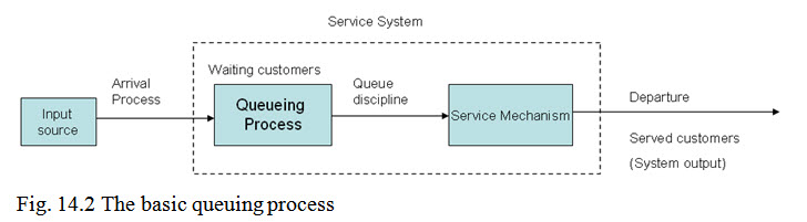
The various elements of the queuing system are: Input source (population), Waiting line (queue), Service discipline, Service mechanism, System output and Customer behaviour.

14.5.1.1. Input source

Two important characteristics of the input source are: (i) its size and (ii) the pattern of arrival.

The size is the total number of customers that might require service from time to time. The size of the input source is generally assumed to be infinite. The railway reservation system, tax / toll both on highway etc. are the example of infinite queue.

The arrival of the customers may be either at a constant rate or at random. Most arrivals in a service system are at random. This is when each arrival is independent of its previous arrivals. The exact prediction of any arrival in random system is not possible. Therefore, the number of arrivals per unit time (rate of arrival) is estimated by Poisson distribution.

14.5.1.2. Queue

A queue is characterized by the maximum permissible number of customers that it contains. Units requiring service enter the system and join a queue. In some service systems only a limited number of customers are allowed in the system and new arrivals are not allowed to join the system unless the number becomes less than the limiting value.

The important characteristics required to study the waiting line are:

(i)   Waiting time: It is the time that a customer spends in the queue before being taken up for service.

(ii)  Service time: It is the time period between two successive services. It may be either constant or variable.

(iii) Waiting time in the system: It implies the time spent by the customer in the queue system. Waiting time in the system = Waiting time + Service time

(iv) Queue length: It implies the number of customers waiting in the queue.

(v) System length: System length is equal to the number of customers in the queue plus those being served.

14.5.1.3. Service discipline and mechanism

Service discipline refers to the order in which the customers waiting in queue are selected for service. It may be first-come-first-served, random or according to some priority procedure. The rules governing order of service may be.

(i) FIFO. First-In-First-Out. (i.e., first-come-first-served): According to FIFO, the customers are served in the order of their arrival. Examples are bank counters, railway reservation counters etc.

(ii) LIFO. Last-In-First-Out. According to LIFO, the items arriving last are taken out first. Example, in big godowns/warehouses, the items arrived last are taken out first.

(iii) SIRO. Service-In-Random-Order. (or Random and priority) Sometimes, certain customers are given priority for service i.e., the arriving customer is chosen for service ahead of some other customers already in the queue. Example: Serious patients are given priority for treatment, vital machines are attended to first in the case of their breakdowns, important orders are given priority in production scheduling.

First-come-first-served (FIFO) is usually implicitly assumed by queuing models unless otherwise stated.

Service mechanism consists of one or more service facility each of which contains one or more parallel service channels.

A server may be a single individual or a group of persons, e.g., a maintenance crew. Furthermore, servers need not even be people, in many cases a server may be a machine or a piece of equipment, e.g., fork lift truck. Service mechanism may vary depending upon the number of service channels, number of servers, number of phases etc. The four basic structures of service mechanism are:

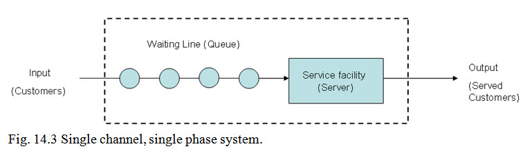
(i) Single Channel Single Phase (Single Queue-Single Server). In this case the arriving units form one queue to be served by a single service facility:

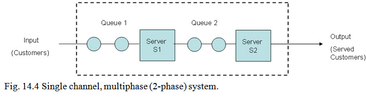
(ii) Single Channel, Multiphase (Single Queue, Multiple Servers in Series). In this case the customers are served at number of servers arranged in series. A two phase service means that once an arrival enters the service, it is served at two stations (or phases one after the other).

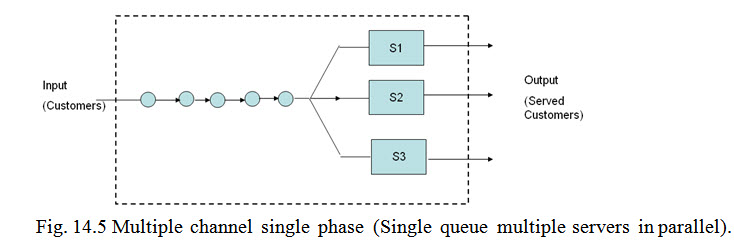
(iii) Multi Channel, Single Phase System (Single Queue, Multiple Servers in Parallel). In this type there is a single queue and multiple servers arranged in parallel as shown in Figure 14.5.

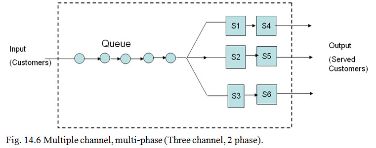
(iv) Multiple Channel, Multiple Phase. In this type there are multiple channels and the customers are served at more than one server as shown in Figure 14.6.

14.5.1.4. System Output

System output refers to the rate at which customers are rendered service. It depends upon service time required by that facility to render service and the arrangement of service facility. The average number of customers that can be served per unit time is called service rate. It can be obtained by constructing service time frequency distribution. Service rate is denoted by letter ‘µ’. Reciprocal of service rate is called service time i.e., Service time =µ^-1

14.5.1.5. Customer Behaviour

Customer behaviour implies that reactions of the typical customers about queuing system of the service mechanism. Typical tendencies of the customers are:

(i) Balking: A new customer refuses to enter the system.

(ii) Reneging: A customer may leave the queue without getting service after waiting sometime.

(iii) Jockeying: A customer may keep on switching from one queue to another, when there are more than one service counters.

(iv) Collusion: The customers in the queue may demand service on their behalf as well as on behalf of others.