Micro Irrigation Systems Design

Lesson 8. Hydraulics of Drip Irrigation System

8.1 Pressure Variation in Irrigation Pipe Line

The major requirement in most situations is that the irrigation system must apply water uniformly over the entire field. The performance of the drip system is related to operating pressure. The uniform water application from a drip emitter requires required desired optimum pressure. Friction loss in pipes and fittings, and differences in elevation cause pressure to vary in a field. Friction loss causes the pressure to decrease in the downstream direction, while changes in elevation can cause either an increase or decrease in pressure due to pipe running on uphill or downhill. The difference in pressure between locations along pipe line can be estimated as

Where

P_d & P_u= pressure at down and upstream positions, respectively, kPa

h_l = energy loss in pipe between the up- and downstream positions, m

ΔZ = elevation difference, m (+ve for uphill & -ve for downhill

The energy loss (h_l) includes head loss due to friction and minor loss, which can be estimated as.

The energy loss (h_l) includes head loss due to friction and minor loss, which can be estimated as.

                                 

where

F =constant; f (number of outlets and method used to estimate, H_f)

H_f = friction loss in pipe between up and downstream locations, m

M_l = minor losses through fittings, m

Major and minor losses are two types of losses that occur in pipe flow.

a) Major losses

Major losses occur while water flow along straight pipes. The universal equation used to calculate friction losses of water flow along a pipe is known as the Hazen-Williams equation, given by

                                

As the length of the pipe increases, the discharge in the pipe decreases due to emission outlets and hence the total energy drop is less than as estimated by the above equation 8.3. For this reason, a reduction factor F is introduced

where,

       H_f (100)= head loss due to friction per 100 meter of pipe length, m/100m

       K = a constant which is 1.22 × 10¹² in metric units

D = inner pipe diameter, mm

C = friction coefficient (indicates inner pipe wall smoothness, the higher the C coefficient, the lower the head loss)

Q = flow rate, L s^-1

The Hazen-Williams equation is valid in a limited range of temperature and flow pattern. In small diameter laterals, the Darcy-Weisbach equation gives better results in calculating head loss due to friction in small diameter lateral pipes. It is given by

                                                                 

where

          H_f = head loss, m                                         L = pipe length, m

          f = Darcy-Weisbach friction factor               V = Flow velocity, m s^-1

          g = gravitation acceleration (9.81, m s^-2)        D = inner pipe diameter, m

Both the Hazen-Williams and Darcy-Weisbach equations include a parameter for the smoothness of the internal surface of the pipe wall. In Hazen-Williams, it is the dimensionless C coefficient and with Darcy-Weisbach the roughness factor f, as the C coefficient is higher, head loss will be lower. On the opposite, in the Darcy-Weisbach equation, higher values of indicate higher head losses.

b) Minor losses

The minor losses through fittings can be estimated or obtained from standard tables available in text books and hydraulics manuals/ hand books. Minor losses are created by the flow at bends and transitions. If the flow velocities are high through many bends and transitions in the system, minor losses can build up and become substantial losses. Minor head losses are expressed as an equivalent length factor that adds a virtual length of straight pipe of the accessory diameter to the length of the pipe under calculation.

The Darcy-Weisbach, Hazen Williams or Scobey equation can be used to compute head loss due to friction, H_f. The general form of these equations can be written as

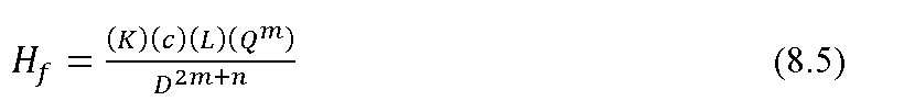                  where

          K = friction factor that depends on pipe material

          L = length of pipe, m

          Q = flow rate,L min^-1

   D = diameter of pipe, mm

c, m, n = constants can be obtained from Table 8.1.

Table 8.1 Constants of friction loss equations

Equations for computing Hf	c	m	n
Darcy-Weisbach	277778	2.00	1.00
Hazen-Williams	591722	1.85	1.17
Scobey	610042	1.90	1.10

(Source: James, 1988)

For the Darcy-Weisbach equation, K is given by the equation

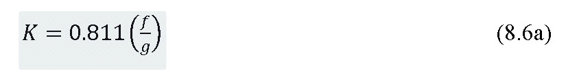                                                where

f = friction factor can be obtained from the Moody diagram

g = acceleration due to gravity (9.81 m s^-2)

K for Hazen-William equation is computed by

                                          

C = Friction coefficient depends on pipe material and diameter.

K for Scobey equation is given by

                                                           

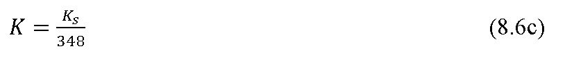
where Ks = friction factor values depends on pipe diameter and pipe material.

There will be less friction loss along a pipe with several equally spaced discharging outlets such as submains and laterals than along a pipe of equal diameter, length, and material with constant discharge (constant discharge means that inflow to the pipe section equals the outflow from the section). This occurs because the quantity of water in the submain or lateral diminishes in the downstream direction because of outlet discharge (i.e. drippers or sprinklers attached with laterals).

The term F in equation (8.2) equals 1 when there are no outlets between the up and downstream locations along a pipe (i.e. discharge along the pipe is constant). Equations 8.7 and 8.8 can be used to estimate F when there is more than one equally spaced outlet. Equation 8.7 is used when the distance from the pipe line to the first outlet is equal to the outlet spacing.

                                                             

Equation 8.8 is used when the distance to first outlet is half of the outlet spacing.

                                  

where

m = Exponent, m (can be obtained from Table 8.1) depending on type of equation involved in estimating H_f.

N = Number of emitters

When the discharge varies widely from outlet to outlet, the Equation (8.1) is applied between successive outlets working from the known pressure to unknown pressure.

8.2      Design of lateral, sub main and main pipes

8.2.1  Lateral pipe Design

Drip irrigation lateral lines are the hydraulic link between the supply lines (main or submain lines) and the emitters. The emission devices can be connected directly to the lateral line (online or inline), mounted on a riser (micro sprinkler, jet) from a buried lateral or attached to the lateral on a tree loop. The lateral line will have hydraulic fittings (tees, unions, etc.,) to connect to the submain or main line. Lateral lines are usually made of LLDPE tubing ranging in diameter 12 mm to 16 mm. Laterals with only one diameter tubing are normally recommended to simplify installation and maintenance and provide better flushing characteristics. The procedures include, determining such lateral characteristics as: flow rate and inlet pressure; locating spacing of manifolds, which in effect sets the lateral lengths; and estimating the differences in pressure within the laterals.

In lateral line design a first consideration is acceptable uniformity of emitter flow or emitter flow variation. If the manufacturers variation is not considered, or assumed to be small, the design can be made to achieve a completely uniform emitter flow by using different emitter sizes or micro tube length (Kenworthy, 1972). In general practice the emitter characteristics are usually fixed and the emitter flow rate is determined by pressure at the emitter in the line.

On fields where the average slope in the direction of the laterals is less than 3%, it is usually most economical to connect laterals to both sides of each manifolds. The manifold should be positioned so that starting from a common manifold connection, the minimum pressures along the pair of laterals are equal. Spacing of manifolds is a compromise between field geometry and lateral hydraulics.

Because of the possibility of laminar, turbulent or fully turbulent flow in drip laterals the Darcy-Weisbach equation should be used to compute head loss due to pipe friction. The Darcy-Weisbach friction factor, f, for small-diameter drip tubing is related to the Reynolds number, R_e the Reynolds number (R_e) is computed with the following equation.

                                                                                  Where,

R_e= Reynolds number (dimensionless);         D = diameter of pipe, cm;

ρ = density of water, g cm^-3;                         V = average velocity, cm s^-1;

μ = viscosity of the fluid, N s m^-2;                 K = unit constant, 10 with these units 

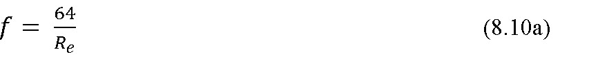
The equation used to compute friction factor (f) depends on the magnitude of N_R. For R_e less than 2000 (laminar flow), the friction factor

                                                              

For R_e between 2000 and 10,0000 (turbulent flow)

                                                                           

For R_e greater than 10,0000 (fully turbulent flow)

                                  

The Hazen-Williams equation with C =150 can also be used to estimate head loss due to pipe friction R_e> 1,00,000.

8.2.2 Submain Design

The submain line hydraulics are similar to that of lateral hydraulics. The submain line is designed to allow approximately the same energy loss as compared to the lateral line for several laterals and submain line. Keller and Karmeli (1975) recommended that the lateral energy loss should be 55 percent and the submain energy loss should be 45 percent of the total allowable energy loss.

The submain design depends on the location of flow or pressure regulation. Energy loss in the submain is directly related to the length of the submain line. The energy loss cannot exceed the allowable limits without lowering uniformity. On particularly steep slopes, each lateral may require individual pressure or flow regulation. In this case the length and diameter of the submain line are determined solely by balancing the energy cost and pipe cost. Since each lateral in this case is regulated, uniformity is independent of submain energy loss provided that submain losses do not interfere with the flow regulation.

The position of the inlet to the submain line depends on the field slope. Usually laterals are placed on contours, if possible with submains running with the prevailing field slope. With sloping submain lines, the inlet is positioned so that the uphill run is shorter than the downhill run. On gently sloping land or level areas the submain inlet should be located near the centre of the submain lines. Submain and main lines should be provided with either manual or automatic flushing valves. Each lateral connection at the submain should have a secondary filter screen to prevent entry of foreign material to the lateral and clogging the emitters.

The submain hydraulics characteristics can be computed by assuming the laterals are analogous to emitters on lateral lines. The hydraulic characteristics of submain and main line pipe are usually taken as hydraulically smooth since PVC pipe are normally used. The Hazen-Williams roughness coefficient (C) usually varies between 140 and 150. The energy loss in the submain can be computed with methods similar to those used for the lateral computations. The energy loss at the lateral connection will depend on the type of connection used, i.e., tee, elbow, bends etc. The total submain energy loss should include energy loss through filters, pressure valves, and other minor losses.

  8.2.3 Mainline Design

Normally, flow or pressure control or adjustment values are provided at the submain inlet. Therefore, energy losses in the mainline should not affect system uniformity. The mainline pipe size is based on economic comparisons of power costs and pipe costs. The mainline pipe size should be selected to minimize the sum of power costs and capital costs over the life time of the pipeline.

Example 8.1 Design a drip irrigation system for a citrus orchard of 1 ha area with length and breadth of 100 m each. Citrus has been planted at a spacing of 5 m ´ 5.5 m. The maximum pan evaporation during summer is 8 mm day^-1. The other relevant data are given below:

Land slope                    = 0.40 % upward from S – N direction

Water source                = A well located at the S–W corner of the field

Soil texture                  = Sandy loam

Clay content                = 18.4 %

Silt                              = 22.6 %

Sand                           = 59.0 %

Field capacity              = 14.9 %

Wilting point               = 8 %

Bulk density               = 1.44 gcc^-1

Effective root zone depth = 120 cm

Wetting fraction          = 0.4

Pan coefficient           = 0.7

Crop coefficient        = 0.8

Solution:

Solution of this Example is taken from Tiwari (2007).

Step I

Estimation of water requirement

Evapotranspiration of the crop = Evaporation from open pan *Pan coefficient Crop coefficient* Crop coefficient

                                                  = 8 * 0.7 *  0.8

                                               = 4.48 mm day^-1

Volume of water to be applied = Area covered by each plant * Wetting fraction *Crop evapotranspiration

                                               = (5 * 5.5) * 0.40 * 4.48

                                               = 49.28 L/day ~ 50 L/day

Step II

Emitter selection and irrigation time

Emitters are selected based on the soil texture and crop root zone system. Assuming three emitters of 4 L h^-1_, placed on each plant root zone in a triangular pattern. These are sufficient to wet the effective root zone of the crop.

Total discharge delivered in one hour = 4 * 3 = 12 L h^-1

Irrigation time = 50 / 12 = 4 h 10 minutes

Step III

Discharge through each lateral 

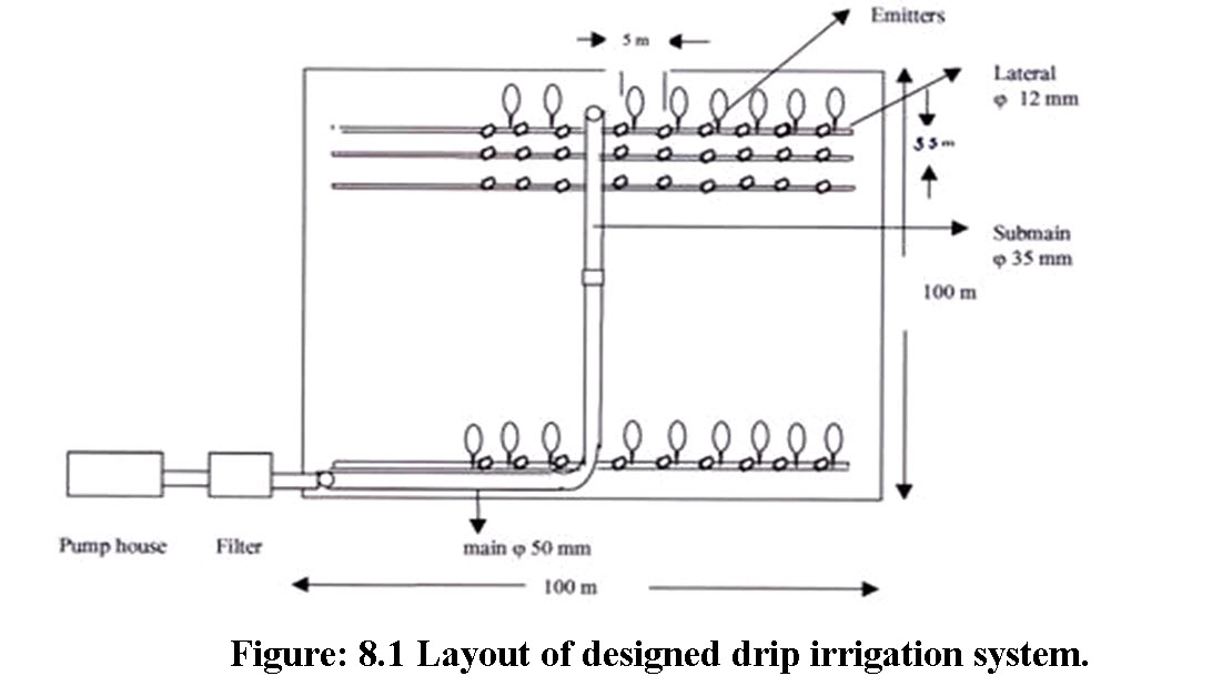
A well is located at one corner of the field. Submains will be laid from the center of field (Fig. 8.1). Therefore, the length of main, sub mains, and lateral will be 50 m, 97.25 m and 47.5 m each, respectively. The laterals will extend on both the sides of the submain. Each lateral will supply water to 10 citrus plants.

Total number of laterals   = (100/5.5) * 2 = 36.36 (Considering 36)

Discharge carried by each lateral, Q_lateral = 10 * 3 * 4 = 120 L h^-1

Total discharge carried by 36 laterals = 120 * 36 = 4320 L h^-1

Each plant is provided with three emitters, therefore total number of emitters will be 36 * 10 * 3 =1080

Step IV

Size of lateral

Once the discharge carried by each lateral is known, then size of the lateral can be determined by using the Hazen- Williams equation.

The reduction factor (F) can be estimated by Equation 8.7

\[F=\frac{1}{{1.852 + 1}}+\frac{1}{{2 \times 30}}+\frac{{\sqrt{1.852-1} }}{{6{{(30)}^2}}}\]

                                            = 0.367

The head loss due to friction in lateral pipe can be estimated using equation 8.3,

   \[{H_f}(100)\] = 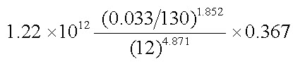= 0.54 m

   \[{H_f}\]= 0.54 * (47.5/100) = 0.26 m

           For D = 16 mm, \[{H_f}\]= 0.063 m

The permissible head loss due to friction is 10% of head of 10 m (head required to operate emitters of 4 L h^-1discharge), which is 1 m. therefore lateral of 12 mm size is adequate and can be chosen.

Step V

Determination of number of manifolds

Assuming the pump discharge = 2.5 L s^-1 = 9000 L h^-1

Discharge carried by each lateral = 120 L h^-1

Number of laterals that can be operated by each manifold = 9000/120 = 75

Therefore, one manifold or sub mains can supply water to all the laterals at a time.

Step VI

Size of sub main

Total discharge through the sub mains =  Q_lateral*Number of laterals

                                                          = 120 * 36

                                                          = 4320 L h^-1 = 1.2 L s^-1

Assuming the diameter of the sub mains as 50 mm. The values of parameter of the Hazen- Williams equation are

\[C\]= 150

\[Q\] = 1.2 L s^-1

\[D\]= 50 mm

 \[K\]= 1.22 * 10¹²

\[{\rm{F}}\] = 0.364

     

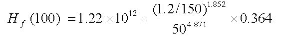
= 0.31 m

\[{H_f}\for 97.25 m of pipe length   = 0.31 * (97.25/100)

       = 0.30 m

Therefore, frictional head loss in the sub mains = 0.30 m

 Pressure head required at the inlet of the sub mains = H _emitter + H_{f lateral} + H_{f sub main} + H _slope

                                                                             = 10 + 0.26 + 0.30 + 0.40

= 10.96 m

Pressure head variation =

                                      = 6.38 %

Estimated head loss due to friction in the sub main is much less than the recommended 20% variation, hence reducing the pipe size from 50 to 35 mm will probably be a good option.

                    = 1.75 m

\[{H_f}\for 97.25 m pipe = 1.75* (97.25/100)

                              = 1.70 m

Pressure head required at the inlet of the sub main = H _emitter + H_{f lateral} + H_{f sub main} + H _slope

                                                                                       = 10 + 0.26 + 1.70 + 0.40

                                                                                      = 12.36 m

Pressure head variation =

                                      = 17%

Pressure head variation lies within the acceptable limit, hence submain pipe of 35 mm is accepted for deisgn.

Step VII

Size of the main line

Assuming the diameter of main as 50 mm

Discharge of main, Q _main = Discharge of sub main, Q_{sub main}

The values of parameter of the Hazen- Williams equation are

 \[C\]= 150

  \[Q\]= 1.2 L s^-1

 \[D\]= 50 mm

 \[K\]= 1.22 ´ 10¹²

\[{H_f}\](100) =

= 0.84 m

\[{H_f}\]for 50 m main pipe = 0.84 ´ (50/100)  = 0.42 m

Step VIII

Determining the horse power of pump

Assuming static head as 10 m, head variation due to uneven field and the losses due to pump fittings, etc. is taken as 10 % of all other losses.

H_local = 10 % of all other loss

Total dynamic head = ( H_emitter + H_{f lateral} + H_{f sub main} + H _slope )+H_{f main}+H_static+H_local

                                 = 12.36 + 0.42 +10 +1.28

                                 = 24.06 m

Pump Horse power(hp)=\[\frac{{H\times Q}}{{75\times{\eta _p}}}\]

where,

\[H\]= Total dynamic head, m

 \[Q\]= Total discharge through main line, L s^-1

\[{\eta _p}\]= Efficiency of pump                                               

hp=\[\frac{{1.2\ \times\ 24.06}}{{75\times 0.60}}\] = 0.64 = 1.0

Hence 1 hp pump is adequate for operating the drip irrigation system to irrigate for 1 ha area of citrus crop.

The design details of components micro irrigation system are estimated as

Length of each lateral= 47.5 m;            Total number of laterals   = 36;

Diameter of lateral = 12 mm;                Length of sub main = 97.25 m;

Number of sub main = 1;                    Diameter of sub main = 35 mm;

Length of main        = 50 m;                Number of main = 1;

Diameter of main     = 50 mm,             Pump horse power required = 1 hp.

 

Refferences:

• James, L. G.  (1988). Principles of Farm Irrigation System Design, John Willey & sons, Inc. New York.

• Keller, J. and Karmeli, D. (1975). Trickle Irrigation Design, Rain Bird Sprinkler Manufacturing Corporation, Glendora, California, USA.

• Kenworthy, A. L. (1972). Trickle Irrigation - The Concept and Guidelines for Use. Research report No. 165, Farm Science., Michigan State University. East Lansing, Michigan.

• Tiwari, K.N. (2007). Pressurized Irrigation, Scientific Publication No. PFDC/IITKGP/1/2007, Precision Farming Development (NCPAH), IIT Kharagpur, India.

Suggested Reading:

• Michael, A. M. (2010). Irrigation Theory and Practice, Vikas Publishing House Pvt. Ltd, Delhi, India.

• James, L. G.  (1988). Principles of Farm Irrigation System Design, John Willey & Sons, Inc. New York.