Micro Irrigation Systems Design

Lesson 22. Terminologies in Economic Analysis

22.1 Types of Costs

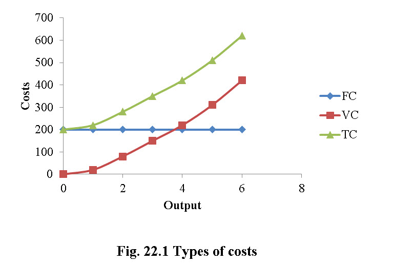
In general, cost or total cost (TC) explains the total economic cost of production of particular goods and comprises of variable costs (VC), which vary according to the quantity of goods produced with inputs such as fertilizer, pesticide, labour etc. plus the fixed cost (FC) which are independent of quantity of goods produced and include inputs such as buildings, rent of land, machinery etc. which cannot be varied over short period of growing season.

i.) Fixed cost (FC)

Fixed costs are also known as annual ownership cost, as they are generally independent of the level of system use as shown in Fig 22.1. Fixed costs include annual depreciation, interest costs and yearly expenditure for taxes and insurance.

ii.) Depreciation

The depreciation means to distribute the cost of given component over the expected life.  Table 22.1 gives the expected useful life of several irrigation system components, has been prepared by the researchers from numerous sources serves as a guideline for estimating depreciation (Thompson et al. 1980). The useful life value is based on 2000 hours use in a year.

Table 22.1 Annual maintenance and repairs, and depreciation guidelines for irrigation system components.

Components	Depreciation	Period (year)	Annual Maintenance and Repairs
Wells and casings	-	20-30	0.5-1.5
Pumping plant structure	-	20-30	0.5-1.5
Pump, vertical turbine
Bowls	16000-20000	8-10	5-7
Column, etc.	32000-40000	16-20	3-5
Pump, centrifugal	32000-50000	16-25	3-5
Power transmission
Gear head	30000-36000		5-7
V-belt	6000	3	5-7
Flat belt, rubber and fabric	10000	5	5-7
Flat belt, leather	20000	10	5-7
Prime movers
Electric motors	50000-70000	25-35	1.5-2.5
Diesel engine	28000	14	5-8
Gasoline engine
Air cooled	8000	4	6-9
Water cooled	18000	9	5-8
Propane engine	28000	14	4-7
Open farm ditches		20-25	1-2
Concrete structure		20-40	0.5-1.0
Pipe, asbestos-cement and PVC buried		40	0.25-0.75
Pipe, aluminium, gated surface		10-12	1.5-2.5
Pipe, steel coated buried		20-25	0.5-0.75
Pipe, steel coated surface		10-12	1.5-2.5
Pipe, steel galvanised surface		15	1.0-2.0
Pipe, wood buried		20	0.75-1.25
Pipe, plastic, trickle, surface		10	1.5-2.5
Sprinkler heads		8	5-8
Trickle emitters		8	5-8
Trickle filters		12-15	6-9
Reservoirs		none	2.0-2.0
Mechanical move sprinklers		12-16	5-8
Continuously moving sprinklers		10-15	5-8

(Source: Thompson et al. 1980)

iii.) Interest costs

Interest is the return from productivity invested capital. When money is borrowed to finance the initial cost of the irrigation system, interest is the money paid for the use of the borrowed money.

iv.)Variable cost (VC)

Variable costs are those which vary as a total cost to the farmer when the output (agricultural production) varies. In fact, variable cost will vary in exactly the same proportion as the output (Fig. 22.1). These include cost of labour, electricity charges etc.

v.)Marginal cost (MC)

Marginal cost is the increase in variable cost associated to a unit increase in production. It can be calculated using eq. 22.1.

MC = ΔTC/ΔQ = ΔVC/ΔQ (for an discrete change of Q)                            

MC= δTC/ δQ= δVC/ δQ (for an infinitesimal change of Q)                         (22.1)

where,

MC = Marginal cost,

Q is the total quantity of goods produced,

VC = Variable cost,

TC = Total cost

If oneimaginesincreasing production one unit at a time, then MC is the cost of last unit produced.

vi.) Average cost (AC)

Average cost is the cost associated to each unit of production, that is, it is how much it costs the average to produce one unit of output. This can be clarified in two ways as shown in Eq. 22.2:

Average variable cost (AVC) = VC / Q

Average total cost (AC) = TC / Q                                                                (22.2)

vii.) Total production function

1^st stage: The total production function is explained through Fig. 22.2.The output (maize yield) increases more than proportionally to the input (seed) increase. This is because the particular input combines better and better with other fixed factors.

2^nd stage: The output (maize yield) increases less than proportionally to the input (seed) increase. This stage must necessarily exist, given that other factors are fixed. For instance increasing quantity of seeds increase output but not indefinitely.

3^rd stage: The output (maize yield) decreases when increasing input (seed) usage (or remains at the same level): when the maximum output is reached, it is impossible to increase further the output, unless other factors are increased.

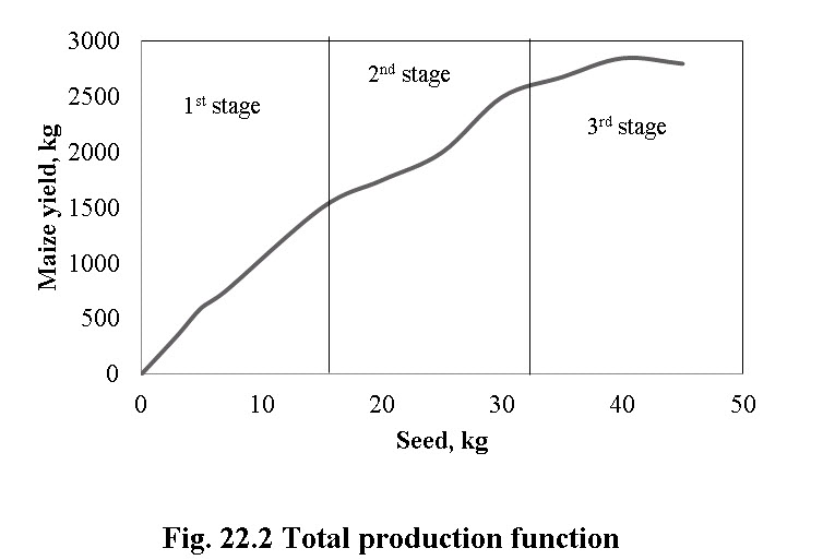
This is expressed as law of diminishing marginal returns: given the fixed factors, production cannot increase indefinitely unless other factors also increase/decrease.

22.2 Supply and Demand

22.2.1Supply

It is the quantity of a commodity that sellers are able and willing to offer for sale atdifferent prices per unit of time.

i)Law of supply: The law of supply states that the quantity of a good offered or willing to offer by the producer/owners for sale, increases with the increase in the market price of the good and falls if vice versa, all other things remaining unchanged.

Supply function expresses the relationship between supply and the factors affecting the producer/supplier to offer goods for sale.

The supply function given below can be expressed as shown in Eq.22.3

Qs = f (P, Prg, S)                                                                              (22.3)

where,

P = price;

Prg = price of related goods; and

S = number of producers.

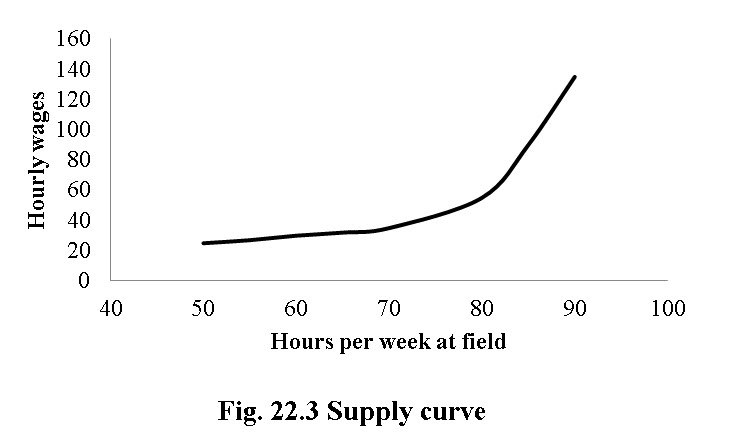
ii) Supply curve

The supply curve is the graphical representation of the supply function and it shows the quantity of a good that the seller is offering or willing to offer at various prices as shown in Fig. 22.3.

 

22.2.2 Demand

Demand is the desire to possess and willingness and ability to pay for particular goods i.e. it’s an effectiveness of desire which explains ability and willingness to pay for a particular commodity. Say, if a person has desire to buy sprinkler system, he has willingness but not the ability to pay for it. Then it becomes a want or a simply wish. So ability and willingness both are important. The major characteristics of demand are (i) ability and willingness to pay for a particular commodity (ii) the demand is always at a given price (iii) demand is always per unit of time.

i.)Law of Demand

It states that as price increases the consumer/buyer will buy less of a particular commodity and vice-versa.

In Table 22.2 the demand of buyers A, B, C and D are the individual demands. Total demand by the fourbuyers is market demand. Therefore, the total market demand is derived by summing upthe quantity demanded of a commodity by all buyers at each price.

Table 22.2 Market demand

Price, Rs.	Buyer A	Buyer B	Buyer C	Buyer D	Market demand
150	2	0	5	0	7
120	5	1	10	3	19
80	9	3	15	9	36
50	12	5	20	12	49
40	17	7	25	13	62

 

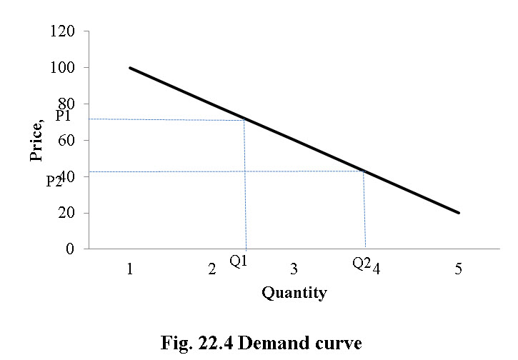
ii.) Demand Curve

Demand curve is a diagrammatic representation of demand schedule. It is a graphical representation of price- quantity relationship. Individual demand curve shows (Fig. 22.4) the highest price which an individual is willing to pay for different quantities of the commodity. As price falls from P₁ to P₂ the quantity demanded increases from Q₁ to Q₂. This is a negative relation between price and quantity, hence the negative slope of the demand schedule; as predicted by the law of demand.

22.3 Net Present Value and Benefit-Cost Ratio

Cost Benefit Analysis (CBA) provides a systematic set of procedures by which a firm or owner can assess whether to undertake a project or an irrigation system or a cropping pattern or a technology when there is choice between mutually exclusive projects or programs or crop.Cost Benefit Analysis is used to assess the value for money of large projects or adaption of new technology in agriculture or change in cropping pattern (Boardman et al. 2006).

The Net Present Value (NPV) of a project simply expresses the difference between the discounted present value of future benefits and the discounted present value of future costs, which is NPV = PV (Benefits) – PV (costs). A positive NPV for a given project signify that project benefits are greater than its costs and vice versa. The formula to calculate the present value (PV) for given future value (FV), interest rate (r), and number of accounting periods (n) is given by Eq.22.4,

                                                                              

 NPV decision rule:

For accept or reject decisions, if NPV ≥ 0, accept, if NPV ≤ 0, reject

Benefit cost ratio decision rule states that

BCR = PV (Benefits)/PV (costs)

Denominator of BCR includes the present value of all project costs, not just the capital costs.

Decision rules:

If BCR ≥ 1 then accept the project, if BCR ≤ 1 then reject the project. It should be clear that when,

NPV ≥ 0, then BCR ≥ 1

and NPV < 0, then BCR < 1

22.4 Internal Rate of Return (IRR)

The internal rate of return of a project is defined as the interest rate at which the net present value of that project equals zero. Let’s consider a case in which cost of financing the project is 15% and IRR is 23%. Now, as the rate of return, the IRR is greater than the cost of financing the project, and thenone should accept the project. If IRR is less than the cost of finance, the project should be rejected. The decision rule for IRR can be given as

When IRR ≥ r, then accept and when IRR < r, then reject.

NPV and IRR give the identical results to accept Vs. reject decisions then considering individual project using Payback period as given in Eq.22.5

                                                   

Example: Suppose forrice production, the initial investment is Rs. 100,000 and net cash inflow is Rs.40000, then the payback period is given by:

100000/40000 = 2.50 years

In the same manner, the payback period for wheat production with initial investment of Rs. 150,000 and net cash inflow of Rs. 58,333 then payback period will be: 150000/58333 = 2.57 years

From above data, one can decide in favour of a project with shorter payback period. Decision can be taken solely based on payback period criteria and does not involve other decision variables.

22.5 Sensitivity Analysis

In engineering economics, sensitivity analysis measures the economic impact resulting from alternative values of uncertain variables that affect the economics of the project. Sensitivity analysis is the study of how the variation in the output of a model (numerical or otherwise) can be approached qualitatively or quantitatively to different sources of variation. Sensitivity analysis can be used to determine model resemblance with the process under study, quality of model definition, factors that mostly contribute to the output variability, region in the space of input factors for which the space of factors for use in a subsequent calibration study, and interaction between factors. Possible situations where sensitivity analysis can be used;

i.) Volume of sales increase by 10%:In this case both the revenue and the labor and inputs would increase by 10%. So the corresponding increase in net income can be analyzed.

ii.)  Prices increase by 10%, but nothing else changes: This may arise if one decides to increase prices and assume that one will be able to still sell the same volume.  Then one can see the corresponding increase in profit/net income.

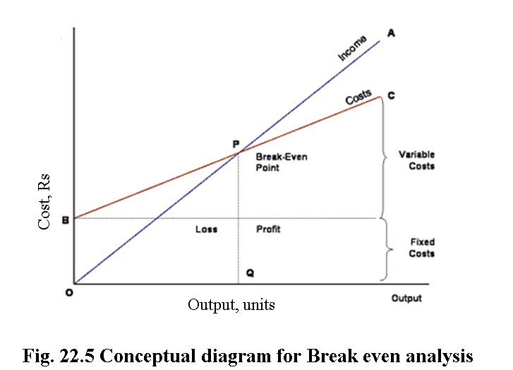
22.6 Break Even Analysis

Break-Even analysis is used to give answers to questions such as “what is the minimum level of sales that ensure the company will not experience loss” or “how much can sales be decreased and the company still continues to be profitable”. Break-even analysis is the analysis of the level of sales at which a company (or a project) would make zero profit. As its name implies, this approach determines the sales needed to break even.

Break-Even point (B.E.P.) is determined as the point where total income from sales is equal to total expenses (both fixed and variable). In other words, it is the point that corresponds to this level of production capacity, under which the company operates at a loss. If all the company’s expenses were variable, break-even analysis would not be relevant. But, in practice, total costs can be significantly affected by long-term investments that produce fixed costs. Therefore, a company in its effort to produce gains for its shareholders – has to estimate the level of goods (or services) sold that covers both fixed and variable costs.

Break-even analysis is based on categorizing production costs between those which are variable (costs that change when the production output changes) and those that are fixed (costs not directly related to the volume of production). The distinction between fixed costs (for example administrative costs, rent, overheads, depreciation) and variable costs (for example production wages, raw materials, sellers’ commissions) can easily be made, even though in some cases, such as plant maintenance, costs of utilities and insurance associated with the factory and production manager’s wages, need special treatment. Total variable and fixed costs are compared with sales revenue in order to determine the level of sales volume, sales value or production at which the business makes neither a profit nor a loss (Diewert, 1984).

(Source: http://www.tutor2u.net/business/production/break_even.html)

In the Fig. 22.5, the line OA represents the variation of income at varying levels of production activity. OB represents the total fixed costs in the business. As output increases, variable costs are incurred, meaning that total costs (fixed + variable) also increase. At low levels of output, Costs are greater than Income. At the point of intersection, P, costs are exactly equal to income, and hence neither profit nor loss is made i.e. Break-even point.

Breakeven point can be calculated using Eq. 22.6

Breakeven point (BEP) = TFC / (SP – VCP)                                         (22.6)
where,

BEP = Breakeven point (units of production)

TFC = Total fixed costs

VCP = Variable costs per unit of production

SP = Selling price per unit of production

References

• Boardman, A. Greenberg, D. Vining, A. and Weimer, D. (2006).Cost-Benefit Analysis: Concepts and Practice, Third Edition, Pearson Prentice Hall, New Jersey.

• Diewert, W. E. (1984). Sensitivity analysis in economics, Comput. and Ops. Res., 11(2):141-156

• Thompson, G. T., Spiess, L. B. and Kridder, J. N. (1980).Farm Resources and System Selection (In Design and Operation of Farm Irrigation Systems. Chapter 3, edited by Jensen M. E.)ASAE Monograph No. 3, Michigan, U.S.A.

• http://www.tutor2u.net/business/production/break_even.htm

 Suggested Reading

• Raju V. T. and Rao, V. S. (1993). Economics of Farm production and Management, Oxford and IBH publishers, New Delhi

• Reddy, S., Subba, Ram, P. Raghu, Sastry,T. V.Neelakanta and Devi, Bhavani (2006). Agricultural Economics.Oxford Publishers, New Delhi.