Lesson 25 Spatial Data

25.1 Neighbourhood Operations

25.1.1 Local Neighbourhood

The general objective of a neighbourhood operation is to analyze the characteristics and/or spatial relationships of locations surrounding some specific (control) locations. Note that the control locations are actually part of the neighbourhood to be analyzed. Neighborhood operations are those that combine a small area or neighborhood of pixels to generate an output pixel. Thus, in fact, spatial interpolation techniques are a type of neighbourhood operations, because they aim to estimate the values at unsampled locations based on values at sampled locations (Carranza, 2009). These are incremental in their behaviour or operation. They work within a small neighbourhood of pixels to change the value of the pixel at the Centre of that neighbourhood, based on the local neighbourhood statistics. Then this process is incremented to the next pixel in the same row and it continued until the whole raster has been processed. Here the dealing data are of implemented 3-D character. Neighbourhood processes can be used to simplify or generalize discrete rasters (Liu and Mason, 2009). Neighbourhood operations applied to raster maps are basically filtering operations. Filtering can be performed in the time domain, frequency domain or spatial domain. Filtering in the spatial domain is a basic function in GIS. Filtering of a raster map involves an equal-sided filter window, also called a “kernel” or “template”, which moves across a raster map one pixel at a time. A filter has an odd number of pixels on each of its sides so that it defines a symmetrical neighbourhood about central pixel. The simplest filter is a square of pixels (Carranza, 2009). The applications of neighborhood operators are many, ranging from digital filters to techniques for sharpening, transforming, and warping images.

Table 25.1. Summary of local pixel statistical operations, their functionality and input/output data format

Statistic	Input format	Functionality	Data type
Variety Mean	Only rasters. If a number is input, it will be converted to a raster constant for that value values occurring in the input rasters	Reports the number of different DN values occurring in the input rasters Reports the average DN value among Output is floating point the input rasters	Output is integer Output is floating point
Standard deviation	Rasters, numbers and constants	Reports the standard deviation of the DN values among the input rasters	Output is floating point
Median Sum Range Maximum Minimum Majority Minority	Only rasters. If a number is input, it will be converted to a raster constant for that value	Reports the middle DN value among the input raster pixel values. With an even number of inputs, the values are ranked and the middle two values are averaged. If inputs are all integer, output will be truncated to integer Reports the total DN value among the input rasters Reports the difference between maximum and minimum DN value among the input raster Reports the highest DN value among the input rasters Reports the lowest DN value among the input rasters Reports the DN value which occurs most frequently among the input rasters. If no clear majority, output ¼ null, for example if there are three inputs all with different values. If all inputs have equal value, output ¼ input Reports the DN value which occurs least frequently among the input rasters. If no clear minority, as majority If only two inputs, where different, output ¼ null. If all inputs equal, output ¼ input. If only one input, output ¼ input	If inputs are all integer, output will be integer, unless one is a float, then the output will be a float

(Source: Liu and Mason, 2009)

25.1.1.1 Distance

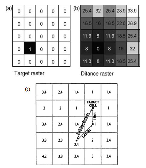
Mapping distance allows the calculation of the proximity of any raster pixel to/from a set of target pixels, to determine the nearest or to gain a measure of cost in terms of distance. Here the value assigned to the output pixel is a function of its position in relation to another pixel. The input is a discrete raster image, in which the target pixels are coded, with a value of 1 against a background of 0 (Fig. 25.1a). This operation involves the use of a straight line distance function, which calculates the Euclidean distance from every pixel to the target pixels (Fig. 25.1b).

The distance transformation transforms a feature or area of raster cells into an area based on given distances. One single distance can be used-for example, 10 m from the well or multiple distances for example 50 m, 100 m, 150 m, 200 m and 250 m from the road for the transformation. The distance transformation geographic information analysis is often used to show the geographic extent of events (e.g., noise from traffic, leaking of oil tanks into the ground) as a thing. In these uses the distances correspond to model or assumed values regarding the process underlying the events. This ability to transform from process to pattern is perhaps the single most important reason for the significance of this geographic information analysis type (Harvey, 2008).

The output pixel values represent the Euclidean distance from the target pixel centers to every other pixel Centre and are coded in the value units of the input raster, usually meters, so that the input raster will usually contain integers and the output normally floating-point numbers. Then the calculated distance raster may then be further reclassified for used as input to more complex multi-criteria analysis or used within a cost-weighted distance analysis.

Fig. 25.1

Spread operation: calculating the distance

Fig. 25.1. (a) An input discrete (binary) raster, (b) the straight line or Euclidean distance calculated from a single target or several targets are coded to every other pixel in an input and (c) Spread operation: calculating the distance. (Source: Malczewski, 1999)

25.1.1.2 Cost pathways

This moving window or kernel procedure is used to derive a cost-weighted distance and cost-weighted direction as part of a least cost pathway exercise. The cost-weighted distance function operates by evaluating each input pixel value of a total cost raster and comparing it with its neighbouring pixels. The average cost between each is multiplied by the distance between them. Cost-weighted direction is generated also from the total cost raster, where each pixel is given a value using a direction-encoded 3×3 kernel, which indicates the direction to the lowest cost pixel value from among its local neighbours. Then these two rasters or surfaces are combined to derive the least cost pathway or route across the raster, to the target.

25.1.1.3 Mathematical morphology

This concept was first developed by Matheron (1975). Mathematical morphology is the combination of map algebra and set theory or of conditional processing and convolution filtering. This concept describes the spatial expansion and shrinking of objects through neighbourhood processing and extends the concept of filtering. These changes include erosion or shrinking, dilation or expansion, opening and closing of raster images. The size and shape of the neighbourhoods used are controlled by structuring elements or kernels which may be of varying size and form. The processing may not be reversible; for instance, after eroding such an image, using an erosion kernel, it is generally not possible to return the binary image to its original shape through the dilation kernel.

Mathematical morphology can be applied to vector point, line and area features but more often involves raster data, commonly discrete rasters and sometimes continuous raster surfaces, such as DEMs. It has also been used in mineral prospection mapping, to generate evidence maps, and in the processing of rock thin section images, to find and extract mineral grain boundaries. This method has applications in raster topology and networks, in addition to pattern recognition, image texture analysis, terrain analysis and also can be used for edge feature extraction and image segmentation.

To illustrate the effects, consider a simple binary raster image showing two classes, shown in Fig. 25.2, the values in the raster of the two classes are 1 (inner, dark grey class) and 0 (surrounding, white class). This input raster is processed using a series of 3×3 structuring elements or kernels (k), which consist of the values 1 and null (instead of 0).

Fig. 25.2

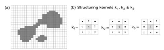
Fig. 25.2. (a) Simple binary raster image (i); and (b) the three structuring kernels (k₁, k₂ and k₃) the effects of which are illustrated in Figs. 25.3–25.5. The black dots in the kernels represent null values.

(Source: Liu and Mason, 2009)

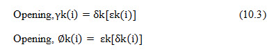
According to the pattern of its neighbouring values, the kernels are passed incrementally over the raster image, changing the central pixel each time. Therefore the incremental neighbourhood operation is similar to spatial filtering but with conditional rather than arithmetic rules controlling the modification of the central value. A simple dilation operation involves the growth or expansion of an object and can be described as:

Where o is the output binary raster, i is the input binary raster and k is the kernel which is centred on a pixel at i, and d indicates a dilation. The Minkowski summation of sets (a b) refers to all the pixels in a and b, in which is the vector sum, and a belongs to set b, and b belongs to set a (Minkowski, 1911). The values of i are compared with the corresponding values in the kernel k, and are modified as follows: the value in o is assigned a value of 1 if the central value of i equals 1, or if any of the other values in k match their corresponding values in i; if they differ, the resultant value in o will be 0. The result of this is only to modify the surrounding outer values by the morphology of the kernel. The effect of a dilation, using kernel k1, is to add a rim of black pixels around the inner shapes and in doing so the two shapes in the binary image are joined into one, both having been dilated, as in Fig. 25.3b.

If the output o₁ is then dilated again using k₁, then a second rim of pixels is added and so on.

By this process, the features are merged into one. Dilation is commonly used to create a map or image that reflects proximity to or distance from a feature or object, such as distance from road networks or proximity to major faults. These distance or ‘buffer’ maps often form an important part of multi-layer spatial analysis. (Source: Liu and Mason, 2009)

Fig. 25.3

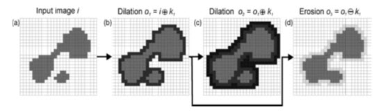
Fig. 25.3. Dilation, erosion and closing: (a) the original image (i); (b) dilation of i using k₁ to produce o₁; (c) dilation of o1 also using k₁ to produce o₂; and (d) erosion of o₁ using k₁ to produce o₃. Notice that o₃ cannot be derived from i by a simple dilation using k₁; the two objects are joined and this effect is referred to as closing. The pixels added by dilation are shown black and those pixels lost through erosion are shown with pale grey tones.

(Source: Liu and Mason, 2009)

A simple erosion operation (a b) has the opposite effect, where is a vector subtraction, so that it involves the shrinking of an object using the Minkowski subtraction, and is described by

where ε indicates an erosion. The values in o are compared with those in k and if they are the same then the pixel is ‘turned off’ i.e. the value in o will be set to 0. The effect of using kernel k₁, is the removal of a rim of value 1 (grey) pixels from the edges of the feature shown in Fig. 25.3b to produce that shown in Fig. 25.3d. It can be noticed that the output o₃, which is the product of the sequential dilation of i, then erosion of o₁, results in the amalgamation of the two original objects and that the subsequent shrinking produces a generalized object which covers approximately the area of the original, an effect known as closing (dilation followed by erosion).

In Fig. 25.4b, an erosion operation is performed on the original i, removing one rim of pixels and causes the feature to be subdivided into two. When this is followed by a dilation, the result is to restore the two features to more or less their original size and shape except that the main feature has been split into two. This splitting is known as an opening and is shown in Fig. 25.4c.

Fig. 25.3

Again, repeated dilations of the features after opening will not restore the features to their appearance in i.

Fig. 25.4

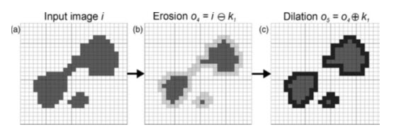
Fig. 25.4. Erosion, dilation and opening: (a) the original image (i); (b) erosion of i using k to produce o4; (c) subsequent dilation of o4, using k1, to produce o5. Note that the initial erosion splits the main object into two smaller ones and that the subsequent dilation does not restore the object to its original shape, an effect referred to as opening. (Source: Liu and Mason, 2009)

Fig. 25.5

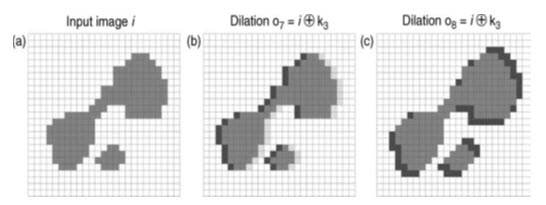
Fig. 25.5. Anisotropic effects: (a) the original image (i); (b) dilation of i using k to produce o6, causing a westward shift of the object; and (c) dilation of i using k3, producing an elongation in the NE-SW directions to produce o7.

(Source: Liu and Mason, 2009)

Closing can be used to generalize objects and to reduce the complexity of features in a raster. Opening can be used to perform a kind of sharpening or to add detail or complexity to the image. Dilation and erosion operations can also be carried out anisotropically in specific directions. Such directional operations are often relevant in geological applications where there is some kind of structural or directional control on the phenomenon of interest.

For example, the effect of kernel k₂ on i is shown in Fig. 25.5a, where the effect is a westward shift of the features by 1 pixel. The effect of kernel k₃ is to cause dilation in the NW–SE directions, resulting in an elongation of the feature (Fig. 25.5b). To consider the effect of mathematical morphology on continuous raster data, we can take the binary image (i) shown in Figs. 25.2–25.5 to represent a density slice through a raster surface, such as an elevation model. In this case, the darker class represent the geographical extent of areas exceeding a certain elevation value. Fig. 25.6a shows the binary image and a line of profile (Fig. 25.6b) across a theoretical surface which could be represented by image (i).The effect of simple dilation and erosion of the surface is shown in Fig. 25.6c.

Fig. 25.6

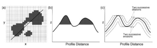
Fig. 25.6 (a) The original input image with the position of a profile line marked; (b) the theoretical cross-sectional profile with the shaded area representing the geographical extent of the darker class along the line shown in (a); and (c) the effect on the profile of dilations and erosions of that surface.

(Source: Liu and Mason, 2009)

Here it can be seen that dilations would have the effect of filling pits or holes, and broaden peaks in the surface, while erosions reduce the peaks or spikes, and widen depressions. Such techniques could therefore be used to correct errors in generated surfaces such as DEMs. But the errors in DEMs cannot be properly corrected by merely smoothing. So for correction of DEM errors a modification of the mathematical morphology technique, known as morphological reconstruction has been proposed. In this case, the original image is used as a mask and the dilations and erosions are performed iteratively on a second version of the same image until stability between the mask and marker images is reached and the image is fully reconstructed and no longer changes, when the holes are corrected (Fig. 25.7).

Since morphological reconstruction is based on repeated dilations, rather than directly modifying the surface morphology, it works by controlling connectivity between areas. The marker could simply be created by making a copy of the mask and either subtracting or adding a constant value. The error-affected raster image is then used as the mask, and the marker is dilated or eroded repeatedly until it is constrained by the mask, i.e. until there is no change between the two, and the process then stops. By subtracting a constant from the marker and repeatedly dilating it, extreme peaks can be removed, whereas by adding a constant and repeatedly eroding the marker, extreme pits would be removed. The extreme values are effectively reduced in magnitude, relative to the entire image value range, in the reconstructed marker image. This technique can be used selectively to remove undesirable extreme values from DEMs.

Fig. 25.7

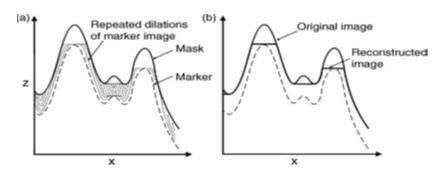
Fig. 25.7. Mechanism of morphological reconstruction of an image, as illustrated by a profile across the image: (a) in this case, by repeated dilations of the marker until it is constrained by the mask image; (b) the extreme peaks are reduced in magnitude in the reconstructed image.

(Source: Liu and Mason, 2009)

25.1.2 Extended neighbourhood

The term ‘extended neighbourhood’ is used to describe operations whose effects are constrained by the geometry of a feature in a layer and performed on the attributes of another layer. These extended neighbourhood operations can be further described as focal and zonal.

If for instance slope angles must be extracted from within a corridor along a road or river, the corridor is defined from one layer and then used to constrain the extent of the DEM from which the slope angle is then calculated (Fig. 25.8).

Fig. 25.8

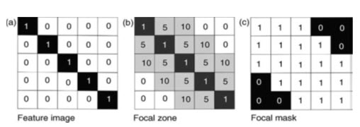
Fig. 25.8. Focal statistics: (a) a binary image representing a linear target feature (coded with a value of 1 for the feature and 0 for the background); (b) a 10m focal image created around the linear feature, where each pixel is coded with a value representing its distance from the feature (assuming that the pixel size is 5m×5 m), areas beyond 10m from the feature remain coded as 0 ; and (c) binary focal zone mask with values of 1 within the mask and zero outside it. This has a similar effect to a dilation followed by a reclassification, to produce a distance buffer. (Source: Liu and Mason, 2009)

25.1.2.1 Focal operations

Working within “neighborhoods” this class of operations implements a moving window algorithm to modify cell values in the input layer (Lein). A focal operation is used for generating corridors and buffers around features. Focal operations are those that derive each new value as a function of the existing values, distances and/or directions of neighbouring locations. The relationships may be defined by Euclidean distance, travel cost, engineering cost or inter-visibility. Such operations could involve measurement of the distance between each pixel (or point) position and a target feature(s). A buffer can then be created by reclassification of the output ‘distance’ layer. This allows specific values to be set for the original target features, with the buffer zones and for the areas beyond the buffers.

25.1.2.2 Zonal operations

These operations are applied to define regions or zones in the input surface. Zones explain collection of cells that exhibit similar attributes which can be created using (1) reclassification calculations based on area, shape or perimeter or (2) categorical overlay developed from binary “cookie cutters” to extract cell values from a raster layer (Lein). A zonal operation also involves the use of the spatial characteristics of a zone or region defined on one layer, to operate on the attribute(s) of a second layer or layers. Since zonal operations most commonly involve two layers, this process falls into the binary operations category. An example is given in Fig. 25.9 where zonal statistics are calculated from an input layer representing the density of forest growth, within the spatial limits defined by a second survey boundary layer, to provide an output representing, in this case, the average forest density within each survey unit. Here it can be seen that the two raster inputs contain integer values but that the output values are floating- point numbers, as is always the case with mean calculations.

Fig. 25.9

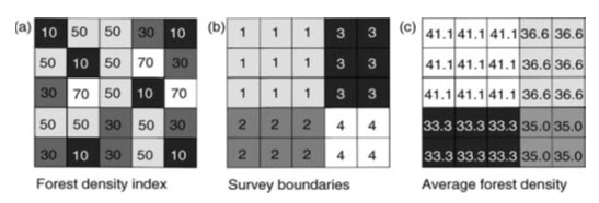
Fig. 25.9. Zonal statistics: (a) forest density integer image; (b) survey boundaries (integer) image; and (c) the result of zonal statistics (in this case a zonal mean) for the same area. Note that this statistical operation returns a non-integer result. (Source: Liu and Mason, 2009)

Keywords: Neighbourhood, raster, pixel, erosion, dilation.

References

Carranza, E. J. M., 2009, Geochemical Anomaly and Mineral Prospectivity Mapping in GIS, pp. 42-44.

Harvey, F., 2008, Primer of GIS: Fundamental Geographic and Cartographic Concepts, The Guilford Press, pp. 258-259.

Malczewski, J., 1999, GIS and Multicriteria Decision Analysis, John Wiley & Sons, pp. 52.

Liu, J. G., and Mason, P. J., 2009, Essential Image Processing and GIS for Remote Sensing, John Willey & Sons, pp. 185-192.

Lein, J. K., Environmental Sensing: Analytical Techniques for Earth Observation, springer, pp. 308-310.

Remote Sensing & GIS Applications

Lesson 25 Spatial Data

(Source: Liu and Mason, 2009)

Suggested Reading

Navigation