Soil Mechanics

LESSON 24. Determination of Coefficient of Consolidation

where H is the thickness of the soil sample, t is required time. T_v is the vertical time factor and can be determine as:

\[{T_v}=\left({{\pi\over 4}}\right){U^2}\quad \quad if\;U \le 60\% \]   %                (24.2)

\[{T_v}=1.781 - 0.933{\log _{10}}(100 - U)\quad \quad if\;U > 60\% \]   %               (24.3)

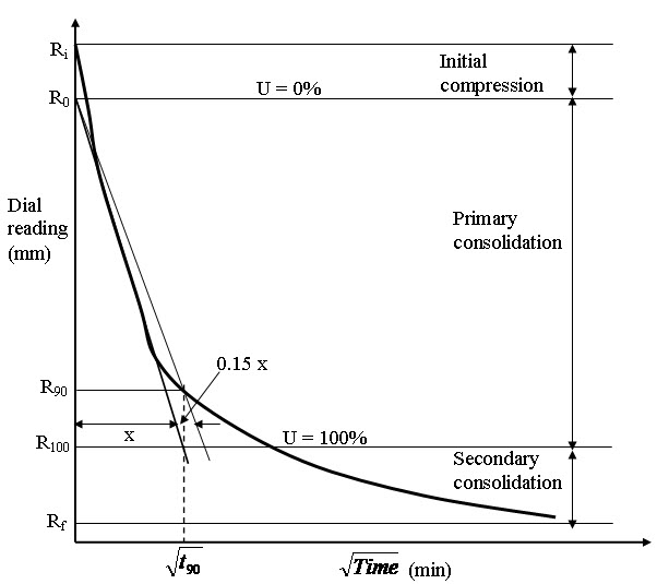
Fig. 24.1. Taylor’s Square Root of Time Fitting Method.

24.2 Casagrande’s Logarithm of Time Fitting Method

From the oedometer test (explained in Lesson 23) the dial reading (settlement) corresponding to a particular time is measured.  From the measured data, dial reading vs time graph can be drawn (as shown in Figure 24.2). Select two points t₁ and t₂ in initial part of the curve such that t₂ = 4 t₁. The points corresponding to the chosen times are marked on the curve. The vertical distance (z) between the two points on the curve is measured. Select another point R₀ such that the vertical distance between that point and point on the curve corresponding to the t₁ time is also z. R₀  is corrected zero reading i.e U = 0%. Determine the U=100% line by drawing two tangents form the straight portion of the curve as shown in Figure 24.2. Once U=0% and 100% lines are identified, U= 50% line is also determined by choosing the middle point between the U=0% and 100% lines. Time (t₅₀) corresponding to the 50% degree of consolidation is determined from the curve. The Coefficient of consolidation (c_v) is determined from Eq.(24.1).

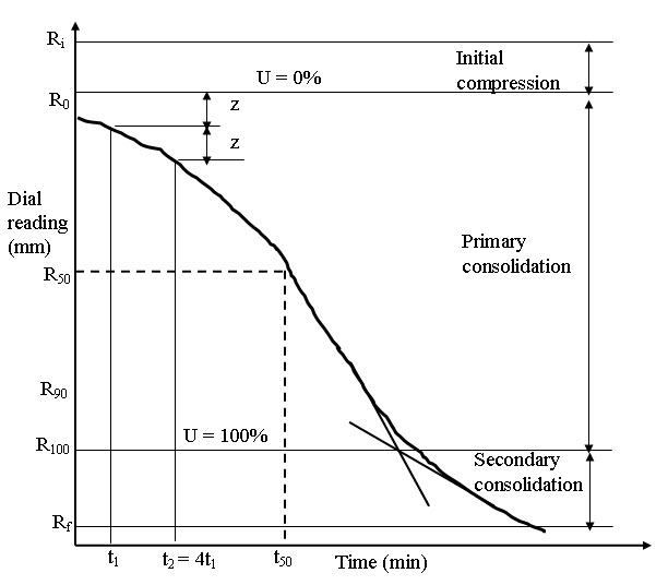
Fig. 24.2. Casagrande’s Logarithm of Time Fitting Method.

Problem 1

 Determine the total settlement of two layered soil system as shown in Figure 24.3. A strip loading of intensity 50 kN/m³ of width 3 m is applied at the ground surface. The water table is at a depth of 1.0 m below ground level.

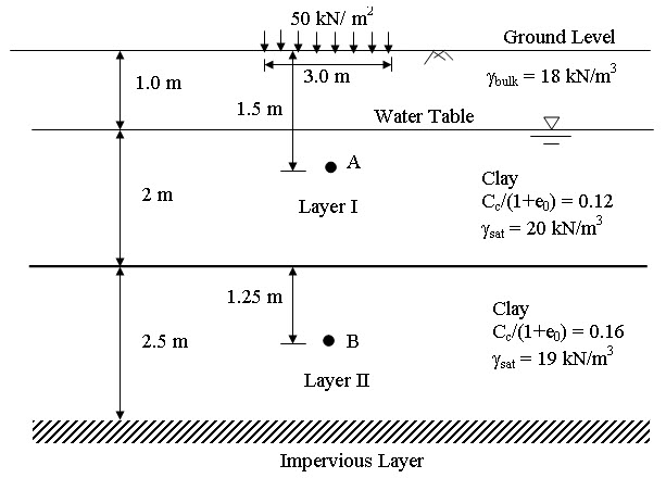
Fig. 24.3. Settlement calculation of two layered soil system.

 Solution:

The thickness of the Layer I and II is 3m and 2.5m, respectively. Choose one point at the middle of each normally consolidated clay layer. Here point A is chosen at a depth of 1.5 m from the ground level (if loading is applied at any depth from the ground level, then the point in the layer I will be chosen as middle of the soil layer in between the loading depth and top of the layer II. In layer II, point will be chosen at the middle of the layer II). The point B is chosen at a depth of 1.25m from the top of the layer II (or 4.25 m below the ground level).

Layer I

At point A,

σ'_v0 = 18 × 1 + (1.5 – 1) × (20 – 10) = 23 kN/m²

Δσ'_v = 50 × 3 /(3+1.5) = 33.33 kN/m² (taking 1:2 distribution of loading)

H₁ = 3m (if loading is applied at a depth, then H₁ will be taken as total thickness of layer I minus the depth of the loading).

\[{S_1}={{{C_c}} \over {1 + {e_0}}}{H_1}{\log _{10}}\left( {{{{{\sigma '}_{v0}} + \Delta {{\sigma '}_v}} \over {{{\sigma '}_{v0}}}}} \right) = 0.12 \times 3 \times {\log _{10}}\left( {{{23 + 33.33} \over {23}}} \right)=140mm\]                     

Layer II

At point B,

σ'_v0 = 18 × 1 + 2 × (20 – 10) + 1.25 (19-10) = 49.25 kN/m²

Δσ'_v = 50 × 3 /(3+4.25) = 20.69 kN/m² (taking 1:2 distribution of loading)

H₂ = 2.5m (if loading is applied at a depth, then H₂ will be taken as total thickness of layer II).

\[{S_2}={{{C_c}} \over {1 + {e_0}}}{H_2}{\log _{10}}\left( {{{{{\sigma '}_{v0}} + \Delta {{\sigma '}_v}} \over {{{\sigma '}_{v0}}}}} \right) = 0.16x2.5x{\log _{10}}\left( {{{49.25 + 20.69} \over {49.25}}} \right)=60.93mm\]

Total settlement = S₁+S₂= 140 +60.93 = 200.93 mm

 

References

Ranjan, G. and Rao, A.S.R. (2000). Basic and Applied Soil Mechanics. New Age International Publisher, New Delhi, India.

 

Suggested Readings

Ranjan, G. and Rao, A.S.R. (2000) Basic and Applied Soil Mechanics. New Age International Publisher, New Delhi, India.

Arora, K.R. (2003) Soil Mechanics and Foundation Engineering. Standard Publishers Distributors, New Delhi, India.

Murthy V.N.S (1996) A Text Book of Soil Mechanics and Foundation Engineering, UBS Publishers’ Distributors Ltd. New Delhi, India.