Site pages
Current course
Participants
General
MODULE 1. Analysis of Statically Determinate Beams
MODULE 2. Analysis of Statically Indeterminate Beams
MODULE 3. Columns and Struts
MODULE 4. Riveted and Welded Connections
MODULE 5. Stability Analysis of Gravity Dams
Keywords
5 April - 11 April
12 April - 18 April
19 April - 25 April
26 April - 2 May
LESSON 4. Deflection of Beam: Direct Integration Technique - 2
4.1 Introduction
In the last lesson we derived the following differential equations.
\[{{{d^2}y} \over {d{x^2}}}=- {M \over {EI}}\] (4.1)
\[{{{d^2}} \over {d{x^2}}}\left( {EI{{{d^2}y} \over {d{x^2}}}} \right)=-{{dV} \over {dx}} \Rightarrow {{{d^2}} \over {d{x^2}}}\left( {EI{{{d^2}y} \over {d{x^2}}}} \right) = q\] (4.2)
In this lesson we will study how to determine the transverse deflection of a beam by solving the above equation by direct integration technique. The procedure is illustrated bellow via several examples.
Example 1
A simply supported beam AB is subjected to a uniformly distributed load of intensity of q as shown in Figure 4.1. Calculate the deflection at the midspan. Flexural rigidity of the beam is EI.
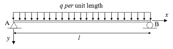
Fig. 4.1.
Solution
The free body diagram of the entire structure is shown in Figure 4.2.
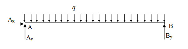
Fig. 4.2.
Applying equilibrium conditions we have,
\[\sum {{F_x}}=0 \Rightarrow {A_x}=0\] (4.3a)
\[\sum {{M_B}}=0 \Rightarrow {A_y}l - ql{l \over 2}=0 \Rightarrow {A_y}={{ql} \over 2}\] (4.3b)
\[\sum {{F_y}}=0 \Rightarrow {A_y} + {B_y} - ql=0 \Rightarrow {B_y}={{ql} \over 2}\] (4.3c)
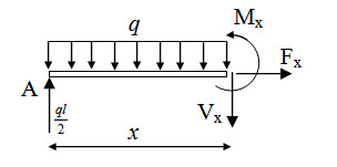
Fig. 4.3.
Using the FBD shown in Figure 4.3 bending moment at a distance x from A is,
\[{M_x}={{ql} \over 2}x - {{q{x^2}} \over 2}\] (4.4)
and equation (4.1) becomes
\[EI{{{d^2}y} \over {d{x^2}}}=- {{ql} \over 2}x + {{q{x^2}} \over 2}\] (4.5)
\[\Rightarrow EI{{dy} \over {dx}}=-{{ql} \over 4}{x^2} + {{q{x^3}} \over 6} + {c_1}\] (4.6)
\[\Rightarrow EIy=-{{ql} \over {12}}{x^3} + {{q{x^4}} \over {24}} + {c_1}x + {c_2}\] (4.7)
where, c1 and c2 are integration constants. In order to evaluate these constants following boundary conditions are used.
y(x = 0) and y(x = l) = 0
Imposing the above boundary conditions we have, \[{c_1}={{q{l^3}} \over {24}}\] and c2=0.
Substituting c1 and c2 in equation (4.7), we have the deflection curve as,
\[y(x)={{qx} \over {24EI}}\left( {{l^3} - 2l{x^2} + {x^3}} \right)\] (4.8)
Deflection at the midspan ( \[x=l/2\] ) is,
\[y(x = l/2)={{5q{l^4}} \over {384EI}}\]
Example 2
A simply supported beam AB is subjected to a linearly varying load as shown in Figure 4.4. Calculate the maximum deflection. Flexural rigidity of the beam is EI.
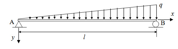
Fig. 4. 4.
Solution
The free body diagram of the entire structure is shown in Figure 4.5.
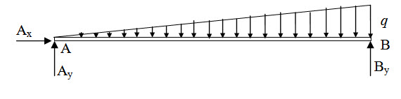
Fig.4.5
Applying equilibrium conditions we have,
\[\sum {{F_x}}=0 \Rightarrow {A_x}=0\] (4.3a)
\[\sum {{M_B}}=0 \Rightarrow {A_y}l - q{l \over 2}{l \over 3} = 0 \Rightarrow {A_y}={{ql} \over 6}\] (4.3b)
\[\sum {{F_y}}= 0\Rightarrow {A_y} + {B_y} - q{l \over 2}=0 \Rightarrow {B_y}={{ql} \over 3}\] (4.3c)
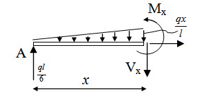
Fig.4.6
Using the FBD shown in Figure 4.3 bending moment at a distance x from A is,
\[{M_x}={{ql} \over 6}x - {{qx} \over l}{x \over 2}{x \over 3} \Rightarrow {M_x}={{ql} \over 6}x - {{q{x^3}} \over {6l}}\] (4.4)
and equation (4.1) becomes
\[EI{{{d^2}y} \over {d{x^2}}}=-{{ql} \over 6}x + {{q{x^3}} \over {6l}}\] (4.5)
\[\Rightarrow EI{{dy} \over {dx}}=-{{ql} \over {12}}{x^2} + {{q{x^4}} \over {24l}} + {c_1}\] (4.6)
\[\Rightarrow EIy=-{{ql} \over {36}}{x^3} + {{q{x^5}} \over {120l}} + {c_1}x + {c_2}\] (4.7)
where, c1 and c2 are integration constants. In order to evaluate these constants following boundary conditions are used.
y(x = 0) and y(x = l) = 0
Imposing the above boundary conditions we have, \[{c_1}={{7q{l^3}} \over {360}}\] and c2 = 0 .
Substituting c1 and c2 in equation (), we have the deflection curve as,
\[y(x) = {{qx} \over {360lEI}}\left( {7{l^4} - 10{l^2}{x^2} + 3{x^4}} \right)\] (4.8)
Where deflection is maximum, \[{{dy} / {dx}} = 0 \Rightarrow x=0.519l\] . Substituting in equation (4.8), we have
\[{\delta _{\max }}=y(x = 0.519l) = 0.00652{{q{l^4}} \over {EI}}\]
Alternative solution using Equation (4.2)
At any distance x from A the intensity of load is \[{q_x} = {{qx} / l}\] . Therefore equation (4.2) becomes,
\[EI{{{d^4}y} \over {d{x^4}}}={{qx} \over l}\] (4.9)
\[\Rightarrow EI{{{d^3}y} \over {d{x^3}}} = {{q{x^2}} \over {2l}} + {c_1}\] (4.10)
\[\Rightarrow EI{{{d^2}y} \over {d{x^2}}} = {{q{x^3}} \over {6l}} + {c_1}x + {c_2}\] (4.11)
\[\Rightarrow EI{{dy} \over {dx}} = {{q{x^4}} \over {24l}} + {c_1}{{{x^2}} \over 2} + {c_2}x + {c_3}\] (4.12)
\[\Rightarrow EIy = {{q{x^5}} \over {120l}} + {c_1}{{{x^3}} \over 6} + {c_2}{{{x^2}} \over 2} + {c_3}x + {c_4}\] (4.13)
Boundary conditions are,
y(x = 0) 0 ; y(x = l) = 0
\[{{{d^2}y} \over {d{x^2}}}(x = 0)=0\] ; \[{{{d^2}y} \over {d{x^2}}}(x = l)=0\] \[\left[ {{\rm{Moment is zero at end}}} \right]\]
Imposing the boundary conditions we have,
\[{c_1}=-{{ql} \over 6}\] ; c2 = 0; \[{c_3}={{7q{l^3}} \over {360}}\] ; c4 = 0.
Substituting c1,c2 ,c3 and c4 in equation (), we have the deflection curve as,
\[y(x)={{qx} \over {360lEI}}\left( {7{l^4} - 10{l^2}{x^2} + 3{x^4}} \right)\]
Where deflection is maximum, \[{{dy}/ {dx}} = 0 \Rightarrow x=0.519l\] . Substituting x = 0.519l in equation (4.8), we have
\[{\delta _{\max }} = y(x = 0.519l) = 0.00652{{q{l^4}} \over {EI}}\]
Suggested Readings
Hbbeler, R. C. (2002). Structural Analysis, Pearson Education (Singapore) Pte. Ltd.,Delhi.
Jain, A.K., Punmia, B.C., Jain, A.K., (2004). Theory of Structures. Twelfth Edition, Laxmi Publications.
Menon, D., (2008), Structural Analysis, Narosa Publishing House Pvt. Ltd., New Delhi.
Hsieh, Y.Y., (1987), Elementry Theory of Structures , Third Ddition, Prentrice Hall.
Last modified: Tuesday, 17 September 2013, 4:20 AM