Site pages
Current course
Participants
General
Module 1: Watershed Management – Problems and Pros...
Module 2: Land Capability and Watershed Based Land...
Module 3: Watershed Characteristics: Physical and ...
Module 4: Hydrologic Data for Watershed Planning
Module 5: Watershed Delineation and Prioritization
Module 6: Water Yield Assessment and Measurement
Module 7: Hydrologic and Hydraulic Design of Water...
Module 8: Soil Erosion and its Control Measures
Module 9: Sediment Yield Estimation/Measurement fr...
Module 10: Rainwater Conservation Technologies and...
Lesson 13 Hydrologic and Hydraulic Design of Recharge Structures
Recharge structures play a very important role in watershed management through artificial groundwater recharge. In most of the cases, recharge structures also result in surface water conservation –discussed in detail in Lesson 19 and Lesson 20 of Module 10. The design of these structures is based on the sound principles of hydrology and hydraulics. In this lesson, we shall discuss the hydrologic and hydraulic design of recharge structures falling under direct methods and surface methods.
13.1 Hydrologic Design as Applied to Recharge Structures
There are three main methods of artificial groundwater recharge as listed below.
Direct methods.
Indirect methods.
Incidental methods.
(A) Direct Methods: Direct methods of recharge can further be subdivided into two main categories as surface methods and sub-surface methods.
(B) Surface Methods: In this method of recharge, water is applied on the permeable ground surface wherein it infiltrates into the unsaturated zone to reach slowly the underground water table. Surface techniques, especially spreading techniques of artificial recharge are most widely used because of their economy and easiness in operation. Various types of spreading techniques are as follows:
Recharge basins
Furrows and ditches
Regulated stream channels
(C) Recharge Basins:
Excavation or building dikes or levees constitute basins [Refer to Fig 13.1]. The shape and size of the basin depends upon topography and availability of land. To reduce deposition of sediments, the water released to the basin should have minimum sediment. This can be achieved by the following measures:
By water diversion to the basin during the non-flood periods, when the suspended sediment is low;
By adding certain chemicals in the water to remove sediments;
By providing Sedimentation basins to hold water before releasing it into the recharge basin.
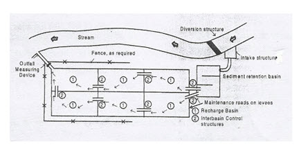
Fig. 13.1. Layout of a typical recharge basin. (Source: Patel & Shah, 2008)
Requirements of Recharge Basin Sites
Knowledge of surface geology downward in the basin and laterally away from the basin;
Considerable knowledge of permeable soil in the basin which permits adequate infiltration rate;
Sufficient knowledge of the unsaturated zone between ground surface and water table.
Furrows and Ditches
This method of recharge is very useful for irregular terrain. Furrows and ditches should be shallow, flat bottomed, and closely spread to obtain maximum water contact area. Gradient of major ditches should be sufficient to carry suspended material through the system so that surface openings are not clogged due to deposition of fine-grained material. The design of furrows and ditches system depends upon the topography and the size of the area. A downstream collecting ditch is necessary to return excess water to the main channel. [Refer to Fig. 13.2].
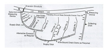
Fig. 13.2. Furrows and ditches for groundwater recharge. (Source: Patel & Shah, 2008)
Regulated Stream Channels
The objective of this method is to extend the time and area over which water is recharged from a natural influent stream channel. It requires upstream storage facilities to regulate stream flows and to enhance infiltration. The flow rate of water should be such that it should not exceed the absorptive capacity of downstream channels. Different types of stream channel regulations include:
Widening, leveling or scarifying a stream channel bed;
Constructing permanent low check dams;
Constructing temporary low check dams of stream bed materials;
Constructing L - shaped finger bikes in straight stream channels and L-shaped hook levees in curved stream channels.
13.2 Hydraulic Design Applied to Recharge Structures
In this section, we shall discuss the theory of artificial groundwater recharge. It will be followed by a discussion on spreading in shallow/ deep phreatic aquifers.
Theory of Artificial Recharge by Spreading
As a variant of induced recharge, the most likely set-up of an artificial recharge scheme consists of a series of spreading ditches and infiltration galleries arranged alternately at equal intervals. For unconfined aquifers which are pervious up to the ground surface, this set-up offers few difficulties. With slight modifications, it may also be applied for artesian aquifers when the confining layer on the top is thin. For confined aquifers covered by thick deposits of less pervious material, recharge must be accomplished by injection wells, having their own problem and possibilities. The simplest construction of parallel spreading ditches and infiltration galleries is shown in Fig. 13.3, where the coefficients of transmissivity (kH) of the aquifer as well as the maximum allowable drawdown (S0) are determined by the local hydro-geological conditions. The other factors indicated in this figure viz., q0, L and w, must be chosen such that the purposes of the recharge scheme are fulfilled.
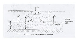
Fig. 13.3. Artificial groundwater recharge with parallel ditches and infiltration galleries (Source: Patel & Shah, 2008)
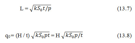
It means an adequate detention time of the recharge water in the sub-soil and no rapid clogging of the spreading basins. When it is provisionally assumed that both the spreading basin and the gallery for groundwater recovery fully penetrate the saturated thickness of the aquifer, these requirements may be formulated mathematically as:
a) Detention time (t)
t = pHL/q0 (13.1)
Or, q0 = pHL/t (13.2)
Here, p is the soil porosity.
b) Maximum allowable drawdown (S0)
S0 = [q0 / (kH)] L (13.3)
Or, q0 = kHS0/L (13.4)
c) Entry rate (ve)
ve = q0 /w (13.5)
or, q0 = ve w (13.6)
The entry rate requirement can always be satisfied by increasing the width of the spreading basin, while the requirements for t and S0 give us the length and flow rate.
With shallow aquifers composed of fine sand, H and k will be small, calling for a short length and a low flow rate, which can best be accomplished using a number of parallel ditches. With deep aquifers built up of coarse sand and high values of aquifer thickness H and hydraulic conductivity k, the length and flow rate may be much greater. The scheme having a number of parallel ditches may again be used, but in plan it tends to be rather square, leading more or less automatically to the recharge scheme of Fig. 13.4. Here a spreading pond is surrounded by a circular battery of wells for recovery of groundwater.
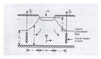
Fig. 13.4. Artificial recharge with a spreading pond surrounded by a circular battery of wells. (Source: Patel & Shah, 2008)
Spreading in Shallow Phreatic Aquifer
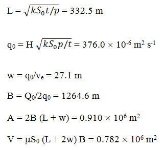
The design procedures to be used in this case can best be demonstrated with an example [Huisman and Olsthorm, 1983]. Consider an aquifer composed of fine sand with a coefficient of permeability (k) = 0.12 ´ 10-3 m/s, a porosity (p) = 0.38, a saturated aquifer thickness before spreading (H0) of 15 m, a maximum allowable rise of water table (S0) = 2 m, giving together an average saturated aquifer thickness during spreading (H) = 16 m. A capacity (Q0) = 30 ´ 106 m3/y or 0.951 m3/s is sought, with a detention time (t) = 8 weeks or 4.84 ´ 106 s and a maximum allowable entry rate (ve) = 0.4 m/d or 4.63 ´ 10-6 m/s. This gives as length and flow rate [Refer to Fig. 13 .3].
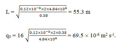
The width of the spreading basin (2w) thus equals
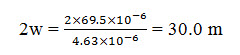
and the combined length of the spreading basins (B) is given by,
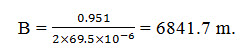
The total area between the infiltration galleries (A) equals
A = 6841.7 ´ [30.0 + (2 ´ 55.3)] = 0.962 ´ 106 m2.
The amount of water in dynamic storage in the pores of the formation between the original and the present water table (V) is given by
V = p S0 (L + 2w) B (13.9)
Out of this volume, a fraction corresponding to the degree of saturation (m/p) can be used. Here μ is the fraction of water voids. With m = 0.25 and the other factors as assumed before,
V = 0.25 ´ 2 ´ (55.3 + 30.0) ´ 6841.7 = 0.292 ´ 106 m3, allowing an interruption in the spreading operations for a period, t = V/Q0 = (0.292 ´ 106)/0.951 = 0.307 ´106 s or 3.55 days.
This period will seldom be adequate to let a wave of polluted river water pass the point of intake. The calculations given above have the attraction of being simple and straight forward, but they have strongly simplified the reality, demanding at this point a number of corrections. The first simplification is the assumption of a constant saturated aquifer thickness (H) in the calculation of the drawdown (S0) given by,
S0 = [q0 / (kH)] L = 2.0 m
Taking into account the variation in water table elevation as well as the recharge by available rainfall (P) [assumed to be temporally uniform at the rate of 400 mm/year or 12.7 ´ 10-9 m/s]. For the case of India and other monsoon climates, this assumption has to be suitably modified. With the commonly used notations, the following is the correct estimation:
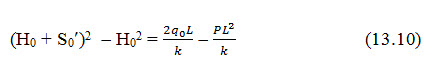
For the case under consideration, the computed maximum drawdown (S0¢) = 1.99 m, which has a negligible difference compared to the value of 2.0 m originally assumed.
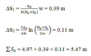
The second simplification concerns the assumption that the spreading ditch fully penetrates the saturated thickness of the aquifer and does so over a width of 2w. To correct this, the spreading ditch is first replaced by a fully penetrating one of zero width, increasing the flow length by an amount w and giving the first additional drawdown (DS1) as:
![]()
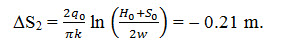
Replacing this ditch by the real one gives the second additional drawdown (ΔS2) as:
Together, we get the total drawdown ( ΣS0) as:
![]()
The third simplification involves the finite length of the spreading ditch. When the area available has a more or less square shape in the top view, the total length of the spreading ditches calculated as 6841.7 m, must be broken up into 6 units, each of a length B = 1140.3 m. This gives a ratio B/L = 1140.3/55.3 = 20.6.
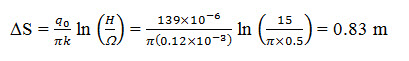
The piezometric level inside the gallery is less than that which corresponds with H0 = 15 m, but this does not affect the water table outside the recharge area. With a number of spreading ditches parallel to one another, the capacity of the gallery (q0) equals 2 ´ 69.5 ´ 10-6 = 139 ´ 10-6 m2s-1, giving for a circular drain of 0.5 m outside diameter (Ω) an additional drawdown due to partial penetration (ΔS) as follows:
To this value, we must add the entrance resistance caused by clogging. Finally, it should be noted that a spreading ditch fully penetrating the saturated thickness of the aquifer over a width of 2w has been assumed. Replacing this ditch by a real one slightly lowers the minimum detention time. But with regard to the improvement in water quality during underground flow, this decrease is compensated by an increase in the average detention time, roughly by a factor of (L + w)/L=1.27 to 6.15 ´ 106 s or 10 weeks.
Spreading in Deep Phreatic Aquifer
The difference in spreading operations for deep and shallow aquifers is not a major one, but it only concerns the layout of the spreading area. Again, this can best be clarified with an example, assuming in this case capacity (Q0) = 30 ´ 106 m3/y = 0.951 m3/s, permeability (k) = 0.4 ´ 10-3 m/s, porosity (p) = 0.38, fraction of water voids (m) = 0.32, maximum allowable entry rate (ve) = 5 cm/h = 13.9 ´ 10-6 m/s, saturated aquifer thickness before spreading (H0) = 60 m, the maximum allowable rise of water table (S0) = 5 m, average saturated aquifer thickness during spreading (H) = 62.5 m, average detention time (t) = 8 months = 21.0 ´ 106 s, to allow when a linear spread in detention time is desired varying between 2 and 14 months. This gives, in the same way as described in the preceding section,
Here we are allowing an interruption in spreading of 9.5 days. The corrected drawdown follows from a uniformly assumed rainfall rate (P) = 400 mm/year = 12.7 ´ 10-9 m/s). For monsoon conditions such as in India, this assumption needs to be suitably modified taking the normal annual rainfall pattern into consideration.
Using Eq. 13.10, the computed maximum drawdown (S0¢) = 4.97 m, which is quite close to the maximum allowable rise of water table (S0) = 5 m.
For a single spreading ditch, bounded at both sides by parallel infiltration galleries has reduction factors for additional flows around the far ends. This reduces 0 to 4.69 m, or well below the maximum allowable value of 5 m.
In the case considered above, the recharge area has a width of 719 m and a length of 1256 m, thus approaching a square area. This indicates a possibility of circular battery of wells. With the usual notation, the design criteria become
(a) Detention time (t), neglecting the soil mass below the spreading pond of dia. (r) at the surface level:
t = pHΠ [(ρ + L)2 -ρ2]/Q0 (13.11)
(b) Drawdown, composed of two terms: S0 = S1 + S2. Here S1 is the flow resistance from the rim of the spreading pond to the concentric battery of wells, calculated from the following Equation
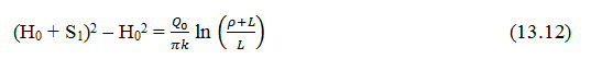
S2 is the flow resistance from the rim of the spreading pond calculated from the following Equation:
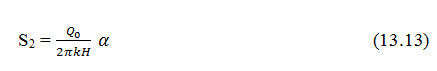
Here, α is tabulated as follows:
|
2ρ/H |
0.01 |
0.1 |
1 |
10 |
100 |
|
α |
308 |
27.6 |
1.58 |
0.088 |
0.0088 |
With sufficient accuracy, α may also be calculated from the equation:
α = e (0.415 - 1.29x + 0.004x^2 + 0.0073 x^3) (13.14)
where, x = ln (2ρ/H).
(c) Entry rate
ve = Q0/(Πρ2) (13.15)
With the same data as in the example above, the following values are obtained:
ρ = 147.6 m [From Eq. 13.15];
L = 390.4 m [From Eq. 13.11];
S1 = 1.99 m [From Eq. 13.12];
S2 = l.28 m [From Eq.s 13.13 and 13.14];
Therefore, S0= S1 + S2 = 3.27 m.
This value for S0 is much smaller than the maximum allowable value of rise in water table of 5.0 m. To remedy this situation, the value of r is to be suitably modified. Accordingly L, S1 and S2 need to be re-calculated so that S0= S1 + S2 will be very to the maximum allowable value of rise in water table of 5.0 m.
The amount of water in dynamic storage (V) is given by,
![]()
Since S is approximated as,

As regard to the pumping equipment of wells for groundwater recovery, the additional drawdown due to point abstraction (ΔSpa) and additional drawdown due to partial penetration (ΔSpp) should be accounted for. Say with 40 wells at an interval of 99m between two wells, the individual capacity = Q0/40 = 23.8[10-3] m3/s. With a screen length of 20 m [i.e., porosity (p) = 20/H0 = 20/60 = 0.333] and an outside dia. of gravel pack [2r0] of 0.60 m, we get
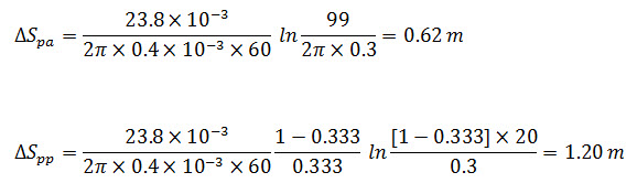
To these values, we must add the additional resistance caused by clogging of well screen and gravel pack.
Keywords: Artificial groundwater recharge, Artificial recharge by spreading, Hydrologic design of recharge structures, Hydraulic design of recharge structures, Groundwater recharge structures.
References
Patel, A. S. and Shah, D. L. (2008). Water Management, New Age International Publishers, pp. 113-121.
Todd, D. K. and Mays, L. W. (2011). Groundwater Hydrology, Wiley India, pp. 547-571.
Suggested Reading
Huisman, L. and Olsthorm, T. N. (1983). Artificial Groundwater Recharge, Pitman Advanced Publishing Program.
http://www.iwmi.cgiar.org/Publications/Water_Policy_Briefs/PDF/wpb01.pdf
Last modified: Thursday, 6 February 2014, 10:25 AM