Electrical Circuits

LESSON 14. Sinusoidal steady state response of circuit

In a network containing energy storage elements, with change in excitation, the currents and voltages change from one state to other state.  The behavior of the voltage or current when it is changed from one state to another is called the transient state.  The time taken for the circuit to change from one steady state to another steady state is called the transient time.  The application of KVL and KCL to circuits containing energy storage elements results in differential, rather than algebraic, equations.  When we consider a circuit containing storage elements which are independent of the sources, the response depends upon the nature of the circuit and is called the natural response.  Storage elements deliver their energy to the resistances.  Hence the response changes with time, gets saturated after some time, and is referred to as the transient response.  When we consider sources acting on a circuit, the response depends on the nature of the source or sources.  This response is called forced response.  In other words, the complete response of a circuit consists of two parts:  the forced response and the transient response.  When we consider a differential equation, the complete solution consists of two parts: the complementary function and the particular solution.  The complementary function dies out after short interval, and is referred to as the transient response or source free response.  The particular solution is the steady state response, or the forced response.  The first step in finding the complete solution of a circuit is to form a differential equation for the circuit.  By obtaining the differential equation, several methods can be used to find out the complete solution.

14.2. DC Response of an R-L Circuit

Consider a circuit consisting of a resistance and inductance as shown in Fig.14.1.  The inductor in the circuit is initially uncharged and is in series with the resistor.  When the switch S is closed, we can find the complete solution for the current.  Application of Kirchhoff’s voltage law to the circuit results in the following differential equation.

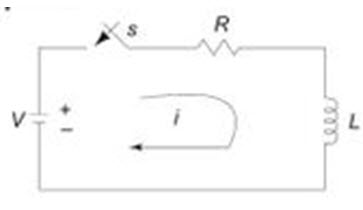
Fig.14.1

\[V=Ri + L{{di} \over {dt}}...................................................\left( {14.1} \right)\]

\[or\,\,{{di} \over {dt}} + {R \over L}i={V \over L}...................................................\left( {14.2} \right)\]

In the above equation, the current t is the solution to be found and V is the applied constant voltage.  The voltage V is applied to the circuit only when the switch S closed.  The above equation is a linear differential equation of first order.  Comparing it with a non-homogeneous differential equation.

\[{{dx} \over {dt}} + Px = K...................................................\left( {14.3} \right)\]

whose solution is

\[x={e^{ - pt}}\,\,f\,K{e^{ + Pt}}\,dt + c{e^{ - Pt}}...................................................\left( {14.4} \right)\]

where c is an arbitrary constant.  In a similar way, we can write the current equations as

\[i=c{e^{ - \left( {R/L} \right)t}} + {e^{ - \left( {R/L} \right)t}}\,\int {{V \over L}{e^{\left( {R/L} \right)t}}\,dt}\]

\[i=c{e^{ - \left( {R/L} \right)t}}\, + {V \over R}...................................................\left( {14.5} \right)\]

To determine the value of c in Eq.14.5, we use the initial conditions.  In the circuit shown in Fig.14.1, the switch S is closed at t=0.  At t=0^-, i.e. just before closing the switch S, the current in the inductor is zero.  Since the inductor does not allow sudden changes in currents, at t=0⁺ just after the switch is closed, the current remains zero.

            Thus at                        t = 0, I  0

Substituting the above condition in Eq.14.5, we have

\[0=c + {V \over R}\]

Hence \[c=-{V \over R}\]

Substituting the value of c in Eq.14.5, we get

\[i={V \over R} - {V \over R}\exp \left( { - {R \over L}t} \right)\]

\[i={V \over R}\,\left( {1 - \exp \left( { - {R \over L}t} \right)} \right)...................................................\left( {14.6} \right)\]

Equation 14.6 consists of two parts, the steady state part V/R, and the transient part (V/R)e^-(R/L)t. When switch S is closed, the response reaches a steady state value after a time interval as shown in Fig.14.2. 

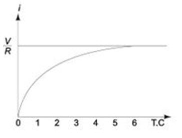
Fig.14.2

Here the transition period is defined as the time taken for the current to reach its final or steady state value from its initial value.  In the transient part of the solution, the quantity L/R is important in describing the curve since L/R is the time required for the current to reach from its initial value of zero to the final value V/R.  The time constant of a function \[{V \over R}e{\,^{ - \left( {{R \over L}t} \right)}}\] is the time at which the exponent of e is unity, where e is the base of the natural logarithms.  The term L/R is called the time constant and is denoted by t

\[\tau={L \over R}\,\,\sec\]

The transient part of the solution is

\[i=-{V \over R}\,\exp \,\left( { - {R \over L}t} \right) = {V \over R}{e^{ - t/\tau }}\]

At one TC, i.e. at one time constant, the transient term reaches 36.8 percent of its initial value.

\[i\left(\tau\right)=-{V \over R}{e^{ - t/\tau }}=-{V \over R}{e^{ - 1}}=-0.368{V \over R}\]

Similarly,

\[i\left( {2\tau } \right)=-{V \over R}{e^{ - 2}}=-0.135{V \over R}\]

\[i\left( {3\tau } \right)=-{V \over R}{e^{ - 3}}=-0.0498{V \over R}\]

\[i\left( {5\tau } \right)=-{V \over R}{e^{ - 5}}=-0.0067{V \over R}\]

After 5 TC, the transient part reaches more than 99 percent of its final value.  In Fig. 14.1, we can find out the voltages and powers across each element by using the current.

            Voltage across the resistor is

\[{\nu _R}=Ri=R \times {V \over R}\left[ {1 - \exp \left( { - {R \over L}t} \right)} \right]\]

\[{\nu _R}=V\left[ {1 - \exp \left( { - {R \over L}t} \right)} \right]\]

Similarly, the voltage across the inductance is

\[{\nu _L}=L{{di} \over {dt}}\]

\[=L{V \over R} \times {R \over L}\exp \left( { - {R \over L}t} \right)=V\,\,\exp \,\left( { - {R \over L}t} \right)\]

The responses are shown in Fig.14.3.

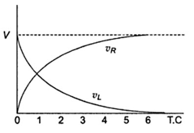
 Fig.14.3

Power in the resistor is

\[{P_R}=\nu _R^i=V\left( {1 - \exp \left( { - {R \over L}t} \right)} \right)\,\left( {1 - \exp \left( { - {R \over L}t} \right)} \right){V \over R}\]

\[={{{V^2}} \over R}\left( {1 - 2\exp \left( { - {R \over L}t} \right) + \,\exp \left( { - {{2R} \over L}t} \right)} \right)\]

Power in the inductor is

\[{P_L}={\nu _L}i = V\;\;\exp \,\left( { - {R \over L}t} \right) \times {V \over R}\left( {1 - \exp \left( { - {R \over L}t} \right)} \right)\]

\[={{{V^2}} \over R}\left( {\exp \left( { - {R \over L}t} \right) - \,\exp \left( { - {{2R} \over L}t} \right)} \right)\]

The responses are shown in Fig.14.4

Fig.14.4

14.3 DC Response of an R-C Circuit

Consider a circuit consisting of resistance and capacitance as shown in Fig.14.5.  The capacitor in the circuit is initially uncharged, and is in series with a resistor.  When the switch S is closed at t=0, we can determine the complete solution for the current.  Application of the Kirchhoff’s voltage law to the circuit results in the following differential equation.

\[V=Ri + {1 \over C}\int {i\,\,dt} ...................................................\left( {14.7} \right)\]

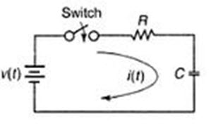
Fig.14.5

By differentiating the above equation, we get

\[0=R{{di} \over {dt}} + {i \over C}...................................................\left( {14.8} \right)\]

or \[{{di} \over {dt}} + {1 \over {RC}}i=0...................................................\left( {14.9} \right)\]

Equation 14.9 is a linear differential equation with only the complementary function.  The particular solution for the above equation is zero.  The solution for this type of differential equation is

i = ce^-t/RC  \[...................................................\left( {14.10} \right)\]

Here, to find the value of c, we use the initial conditions.

In the circuit shown in Fig.14.6, switch S is closed at t = 0.  Since the capacitor never allows sudden changes in voltage, it will act as a short circuit at t=0⁺.  So, the current in the circuit at t=0⁺ V/R

\[At\,t = 0,\,the\,\,current\,i={V \over R}\]

Substituting this current in Eq. 14.10, we get

\[{V \over R}=c\]

The current equation becomes

\[i={V \over R}{e^{ - t/RC}}...................................................\left( {14.11} \right)\]

When switch S is closed, the response decays with time as shown in Fig.14.6.

            In the solution, the quantity RC is the time constant, and is denoted by t,

            where t = RC sec

After 5 TC, the curve reaches 99 percent of its final value.  In fig. 14.5, we can find out the voltage across each element by using the current equation.

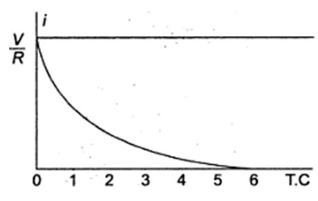
 Fig.14.6

Voltage across the resistor is

\[{\nu _R}=Ri=R \times {V \over R}{e^{ - \left( {1/RC} \right)t}};\,\nu R = V{e^{ - t/RC}}\]

Similarly, voltage across the capacitor is

\[{\nu _C}={1 \over C}\int {i\,\,dt}\]

\[={1 \over C}\int {{V \over R}{e^{ - tRC}}\,dt}\]

\[=-\left( {{V \over {RC}} \times RC\,{e^{ - t/RC}}} \right) + \, = \, - V{e^{ - t/RC}} + c\]

At t=0, voltage across capacitor is zero

c = V

\n_c = V(1 – e^-t/RC)

The responses are shown in Fig.14.7.

Power in the resistor

\[{P_R}=\nu _R^i=V{e^{ - t/RC}} \times {V \over R}{e^{ - t/RC}}={{V2} \over R}{e^{ - 2t/RC}}\]

Power in the capacitor

\[{P_C}=\nu _c^i=V\left( {1 - {e^{ - t/RC}}} \right){V \over R}{e^{ - t/RC}}\]

\[={{{V^2}} \over R}\left( {{e^{ - 1/RC}} - {e^{ - 2t/RC}}} \right)\]

The responses are shown in Fig.14.8.

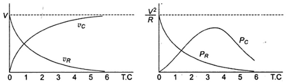
Fig.14.7                                               Fig.14.8

14.4. DC Response of an R-L-C Circuit

Consider a circuit consisting of resistance, inductance and capacitance as shown in Fig.14.9.  The capacitor and inductor are initially uncharged, and are in series with a resistor.  When switch S is closed at t=0, we can determine the complete solution for the current. 

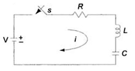
Fig14.9

Application of Kirchhoff’s voltage law to the circuit results in the following differential equation.

\[V=Ri + L{{di} \over {dt}} + {1 \over C}\int {idt} ...................................................\left( {14.12} \right)\]

By differentiating the above equation, we have

\[0=R{{di} \over {dt}} + L{{{d^2}i} \over {d{t^2}}} + {1 \over c}i...................................................\left( {14.13} \right)\]

or \[{{{d^2}i} \over {d{t^2}}} + {R \over L}\,{{di} \over {dt}} + {1 \over {LC}}i=0...................................................\left( {14.14} \right)\]

The above equation is a second order linear differential equation, with only complementary function.  The particular solution for the above equation is zero.  Characteristic equation for the above differential equation is

\[\left( {{D^2} + {R \over L}D + {1 \over {LC}}} \right)=0...................................................\left( {14.15} \right)\]

The roots of Eq.14.15 are

\[{D^1},{D^2}=-{R \over {2L}} \pm \sqrt {{{\left( {{R \over {2L}}} \right)}^2} - {1 \over {LC}}}\]

By assuming \[{K_1}=-{R \over {2L}}and\,\,{K_2}=\sqrt {{{\left( {{R \over {2L}}} \right)}^2} - {1 \over {LC}}}\]

D₁ = K₁ + K₂  and D₂ = K₁ – K₂

Here K₂ may be positive, negative or zero.

K₂ is positive, when \[{\left( {{R \over {2L}}} \right)^2}\, > 1/LC\]

The roots are real and unequal, and give the over damped response as shown in Fig.14.10.  Then Eq.14.14 becomes

\[\left[ {D - \left( {{K_1} + {K_2}} \right)} \right]\,\left[ {D - \left( {{K_1} - {K_2}} \right)} \right]\,\,i=0\]

The solution for the above equation is

\[i={c_1}{e^{\left( {K1 + K2} \right)t}} + {c_2}{e^{\left( {K1 - K2} \right)t}}\]

The current curve for the overdamped case is shown in Fig.14.10.

K₂ is negative, when (R/2L)²< 1/LC

The roots are complex conjugate, and give the underdamped response as shown in Fig.14.11.  Then Eq. 14.14 becomes

\[\left[ {D - \left( {{K_1} + j{K_2}} \right)} \right]\,\left[ {D - \left( {{K_1} - j{K_2}} \right)} \right]\,\,i=0\]

The solution for the above equation is

\[i={c_1}{e^{K1t}}\left[ {{e_1}\,\,\cos \,{K_2}t + {c_2}\,\sin \,{K_2}t} \right]\]

The current curve for the underdamped case is shown in Fig.14.11.

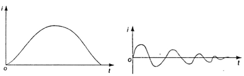Fig. 14.10                                       Fig. 14.11

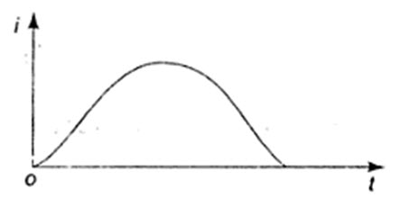
Fig14.12

K₂ is zero, when (R/2L)² = 1/LC

The roots are equal, and give the critically damped response as shown in Fig.14.12.

Then Eq.14.14 becomes

(D-K₁) (D-K₁)i = 0

The solution for the above equation is

\[i={e^{{K_1}t}}\left( {{c_1} + {c_2}t} \right)\]

The current curve for the critically damped case is shown in Fig.14.12.