Gulley & Ravine Control Structures 3(2+1)

Lesson 12 Runoff Estimation– SCS Curve Number Method

12.2 Determination of Curve Number

The SCS-CN method is based on the water balance equation and two fundamental hypotheses. The first hypothesis equates the ratio of the actual amount of direct surface runoff (Q) to the total rainfall (P) (or maximum potential surface runoff) to the ratio of the amount of actual infiltration (F) to the amount of the potential maximum retention (S). The second hypothesis relates the initial abstraction (Ia) to the potential maximum retention, thus the SCS-CN method consists of:

(a) Water Balance Equation:                  

 P = I_a + F + Q                                          (12.1)

(b) Proportional Equality Hypothesis:

  Q/P-Ia = F/S                                            (12.2)

(c) I_a -S hypothesis

I_a= λ S                                               (12.3)

Where P= total rainfall; Ia =initial abstraction; F= cumulative infiltration excluding Ia; Q= direct runoff; and S= potential maximum retention or infiltration.

Combining equations 12.1 and 12.2, it becomes

Q = (P - I_a)²/(P - I_a + S)                                (12.4)

Equation is valid for P ≥ Ia. For λ = 0.2, the equation can be written as:

Q = (P - 0.2 S)²/(P + 0.8 S)                         (12.5)

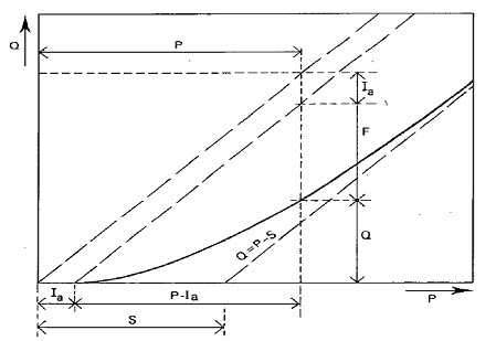
Fig. 12.1. Accumulated runoff Q versus accumulated rainfall P according to the Curve number Method. (Source: http://edepot.wur.nl/183157)

Thus the existing SCS-CN method is a one parameter model for computing surface runoff from daily storm rainfall, for the method was originally developed using daily rainfall-runoff data of annual extreme flows.  S is a constant and is the maximum difference of (P-Q) that can occur for the given storm and watershed condition. S is limited by either the rate of infiltration at the soil surface or the amount of water storage available in the soil profile, whichever gives the smaller S value. Since parameter S can vary in the range of 0 ≤ S ≤ ∞, it is mapped into a dimensionless curve number(CN), varying in a more workable  range 0 ≤ CN ≤ 100, as follows: (Actually, to make Eq. 12.6 mathematically workable, the CN limit should be 0 < CN ≤ 100)

S = (1000/CN) -10                                               (12.6)

The underlying difference between S and CN is that the former is a dimensional quantity (L) whereas the latter is a non-dimensionless quantity. The CN theoretically varies from 0 to 100.

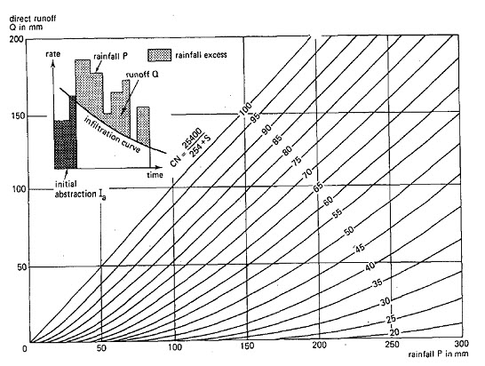
Fig. 12.2. Graphical solution of equation 12.4 showing runoff depth Q as a function of rainfall depth P and curve number. Source: http://edepot.wur.nl/183157)

12.3 Factors Affecting SCS Curve Number

The Curve Number is a dimensionless parameter indicating the runoff response characteristic of a drainage basin. In the Curve Number Method, the CN is related to land use, land treatment, hydrological condition, hydrological soil group, and antecedent soil moisture condition in the drainage basin.

(a) Land Use or Cover

Land use represents the surface conditions in a drainage basin and is related to the degree of cover. In the SCS method, the following categories are distinguished:

Fallow- is the agricultural land use with the highest potential for runoff because the land is kept bare;  Row crops- are field crops planted in rows far enough apart that most of the soil surface is directly exposed to rainfall; Small grain- planted in rows close enough that the soil surface is not directly exposed to rainfall; Close-seeded legumes or rotational meadow- are either planted in close rows or broadcasted. This kind of cover usually protects the soil throughout the year; Pasture range- is native grassland used for grazing, whereas meadow is grassland protected from grazing and generally mown for hay; Woodlands- are usually small isolated groves of trees being raised for farm use.

(b) Practice in relation to Hydrological Condition

Land treatment applies mainly to agricultural land uses. It includes mechanical practices such as contouring or terracing, and management practices such as rotation of crops, grazing control, or burning.

Rotations are planned sequences of crops (row crops, small grain, and close-seeded legumes or rotational meadow). Hydrologically rotations range from poor to good. Poor rotations are generally one-crop land uses (monoculture) or combinations of row crops, small grains, and fallow. Good rotations generally contain close-seeded legumes or grass.

For grazing control and burning (pasture range and forest), the hydrological condition is classified as poor, fair, or good. Pasture range is classified as poor when heavily grazed and less than half the area is covered; as fair when not heavily grazed and between one-half to three-quarters of the area is covered; and as good when lightly grazed and more than three-quarters of the area is covered. Woodlands are classified as poor when heavily grazed or regularly burned; as fair when grazed but not burned; and as good when protected from grazing.

(c) Hydrological Soil Group

Soil properties greatly influence the amount of runoff. In the SCS method, these properties are represented by a hydrological parameter: the minimum rate of infiltration obtained for a bare soil after prolonged wetting. The influence of both the soil’s surface condition (infiltration rate) and its horizon (transmission rate) are thereby included. This parameter, which indicates a soil’s runoff potential, is the qualitative basis of the classification of all soils into four groups. The Hydrological Soil Groups, as defined in the SCS-CN method, are:

Group A:  Soils having high infiltration rates even when thoroughly wetted and a high rate of water transmission. Examples are deep, well to excessively drained sands or gravels.

Group B:  Soils having moderate infiltration rates when thoroughly wetted and a moderate rate of water transmission. Examples are moderately deep to deep, moderately well to well drained soils with moderately fine to moderately coarse textures.

Group C:  Soils having low infiltration rates when thoroughly wetted and a low rate of water transmission. Examples are soils with a layer that impedes the downward movement of water or soils of moderately fine to fine texture.

Group D:  Soils having very low infiltration rates when thoroughly wetted and a very low rate of water transmission. Examples are clayey soils with a high swelling potential, soils with a permanently high water table, soils with a clay pan or clay layer at or near the surface, or shallow soils over nearly impervious material.  Table 12.1 shows Land use categories and associated curves number, according to soil group; commercial land has different curve number.

Table 12.1. Land Use Categories and Associated Curve Numbers

Description	Average % Impervious	Curve Number by Hydrologic Soil Group				Typical Land Uses
		A	B	C	D
Residential (High Density)	65	77	85	90	92	Multi-family Apartments, Trailer Parks
Residential (Med. Density)	30	57	72	81	86	Single-Family, Plot Size 0.1 to 0.4 ha
Residential (Low Density)	15	48	66	78	83	Single-Family, Plot Size 0.4 ha and Greater
Commercial	85	89	92	94	95	Strip Commercial, Shopping Centers, Convenience Stores
Industrial	72	81	88	91	93	Light Industrial, Schools, Prisons, Treatment Plants
Disturbed/Transitional	5	76	85	89	91	Gravel Parking, Quarries, Land Under Development
Agricultural	5	67	77	83	87	Cultivated Land, Row crops, Broadcast Legumes
Open Land	5	39	61	74	80	Parks, Golf Courses, Greenways, Grazed Pasture
Meadow	5	30	58	71	78	Hay Fields, Tall Grass, Un-grazed Pasture
Woods (Thick Cover)	5	30	55	70	77	Forest Litter and Brush adequately cover soil
Woods (Thin Cover)	5	43	65	76	82	Light Woods, Woods-Grass combination, Tree Farms
Impervious	95	98	98	98	98	Paved Parking, Shopping Malls, Major Roadways
Water	100	100	100	100	100	Water Bodies, Lakes, Ponds, Wetlands

(Source: http://proceedings.esri.com/library/userconf/proc00/professional/papers/pap657/p657.htm)

(d) Antecedent Moisture Condition

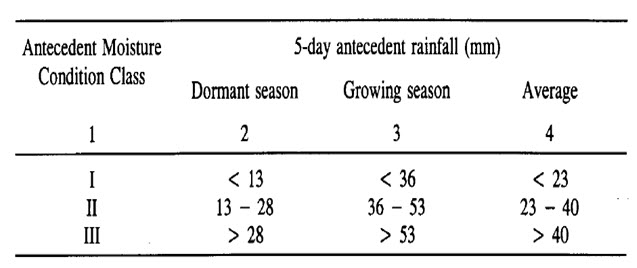
The soil moisture condition in the drainage basin before runoff occurs is another important factor influencing the final CN value. In the Curve Number Method, the soil moisture condition is classified in to three Antecedent Moisture Condition (AMC) Classes:

AMC I: The soils in the drainage basin are practically dry (i.e. the soil moisture         content is at wilting point).

AMC II: Average condition.

AMC III: The soils in the drainage basins are practically saturated from antecedent rainfalls (i.e. the soil moisture content is at field capacity).

These classes are based on the 5-day antecedent rainfall (i.e. the accumulated total rainfall preceding the runoff under consideration), as illustrated in Table 12.2. In the original SCS method, a distinction was made between the dormant and the growing season to allow for differences in evapotranspiration.

Table 12.2. Seasonal rainfall limits for AMC classes (after soil conservation Service, 1972)

(Source: http://edepot.wur.nl/183157)

(e) Agricultural Management Practices

Agricultural management system involves different types of tillage, vegetation, and surface cover. Moldboard Plough increases soil porosity from 10-20%, depending on the soil texture and, in turn, increases infiltration rates as compared to those for the non-tilled soils. Also, an increase in the organic matter content in the soil lowers the bulk density or increases porosity, and hence increases infiltration and in turn, decreases the runoff potential.

(f) Initial Abstraction and Climate

The initial abstraction consists of interception, surface detention, evaporation, and infiltration. The water held by interception, surface detention, and the infiltration at the beginning of a storm finally goes back to atmosphere through evaporation. The effect of the climatic condition of watershed is accounted for by the existing SCS-CN method in terms of the initial abstraction. It is the amount of initial abstraction for a given rainfall amount in watershed. Thus the initial abstraction reduces the runoff potential of the watershed and the curve number.

(g) Rainfall Intensity and Duration and Turbidity

A high intensity rainfall or raindrop breaks down the soil structure to make soil fines move into the soil surface or near-surface pores, leading to the formation of crust that impedes infiltration. The crust formation actually decreases the effective soil depth responsible for infiltration and also the soil porosity, decreases S or increases CN. It is for this reason that a fallow land exposed to rain, produce a higher runoff for a given rainfall amount than does the unexposed or covered land. The term turbidity refers to impurities of water that affect infiltration by the process of clogging of soil pores and consequently, affecting the soil conductivity or ease with which water is transmitted into the soil. The contaminated water with dissolved minerals, such as salts, affects the soil structure and consequently, infiltration.

Table 12.3. Rainfall depth and corresponding direct runoff depth as a function of rainfall duration and AMC condition for a design return period of 10 years

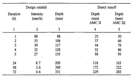
(Source: http://edepot.wur.nl/183157)

12.4 Advantage, Scope and Limitation of SCS-CN Method

• The SCS-CN method has several advantages over other methods.

• It is a simple conceptual method for estimation of the direct runoff amount from a storm rainfall amount, and it is well supported by empirical data.

• The method relies on only one parameter, the curve number CN, which is a function of the major runoff-producing watershed characteristics.

• It is fairly well documented for its inputs (soil, land use/treatment, surface condition, and antecedent moisture condition),

• Its features are readily grasped, well establish, and accepted for use in the United States and other countries.

Limitation

• It does not contain any expression for time and ignore the impact of rainfall intensity and its temporal distribution.

• Time was incorporated in the method because (a) sufficiently reliable data were not available to describe infiltration rates for a wide range of complexes and (b) there was no reliable method available for distributing rainfall in time.

• The SCS-CN method has evolved as a result of research and field monitoring over the years. In many situations, it has given acceptable results. Its further refinement has been a continuous process.

• There is lack of clear guidance on how to vary antecedent moisture condition, especially for lower curve numbers and rainfall amount.

• The method was originally developed for agricultural sites; it performs best on these watersheds, fairly on range sites, and poorly in forest sites.

Prediction Errors Related to the Use of Single Composite CN Values

Grove et al. (1998) in their study investigated the effect of using single composite CN values instead of weighted runoff estimates, indicating that significant errors in runoff estimates can occur when composited rather than distributed CN are used. Lantz and Hawkins (2001) also discussed the possible errors caused by the use of a single composite CN value. The main reason for the errors produced using the composite CN value instead of weighted-Q is the non-linear form of the SCS-CN formula.

Scope of the SCS-CN concept in hydrology

The existing SCS-CN method has been widely used for computing the direct runoff volume from a given rainfall amount. Apart from such an application the method has also been applied to long term hydrologic simulation but only to a limited extent.

1. Computation of Infiltration and DSRO (direct surface runoff) Volumes

The determination of infiltration and runoff volumes is vital to watershed management activities. For computing infiltration and runoff using the SCS-CN, the pertinent parameters are potential maximum retention, S, or curve number, CN.

2. Computation of Infiltration Rates

The problem of computing infiltration rates has been recognized and has been discussed in hydrologic literature. Although the SCS-CN method is construed as an infiltration model, it has not yet been employed in field for computing infiltration rates.

Time-distributed event-based hydrologic simulation

Flood studies often require determination of the peak flow rate and the time of concentration. The lack of short-term real time data can be attributed to the development of the SCS-CN method-based infiltration model with a routing mechanism which will make it possible to compute runoff rates at discrete times during a storm.

3. Long Term Hydrological Simulation

Long term hydrologic simulation is required for analyses of water availability. The SCS-CN method has witnessed only a few applications. With the enhanced understanding of the SCS-CN parameters, it is possible to reasonably simulate daily flows for a much longer period, applying the soil moisture balance.

4. Sediment yield

Sediment has been characterized as the largest carrier of pollutants to receiving water bodies. Much of the sediment carried by streams originates in upland areas. Many methods have been developed for estimation of erosion and sediment yield from agriculture, urban and rural watersheds. One of the most popular methods is the empirically derived universal soil loss equation (USLE). A close examination of this equation suggested that the SCS-CN methodology can be employed to derive a sediment yield equation which is similar to USLE.