Soil Mechanics 3(2+1)

LESSON 6. Stress in Soil due to applied load

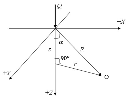
Fig. 6.1. Boussinesq’s stresses.

The vertical stress (σ_z) at a point ‘O’ within the soil with radial distance ‘R’ from the point of application of the concentration load Q can be determined as:

\[{\sigma _Z}={{3Q} \over {2\pi {z^2}}}{\cos ^5}\alpha\]                       (6.1)

The shear stress (t_rz) at a point ‘O’ within the soil with radial distance ‘R’ from the point of application of the concentration load Q can be determined as:

\[{\tau _{rz}}={{3Q} \over {2\pi {z^2}}}{\cos ^4}\alpha \sin \alpha\]                (6.2)

where z and r are the depth and horizontal distance of the point ‘O’ from the point of application of the concentration load Q, respectively.

 Now,

\[\cos \alpha=\frac{z}{R}=\frac{z}{{{{\left({{r^2}+{z^2}}\right)}^{\frac{1}{2}}}}}\]              (6.3)

Thus, Eq. (6.1) can be written as:

\[{\sigma _Z}=\frac{{3Q}}{{2\pi }}\frac{{{z^3}}}{{{R^5}}}=\frac{{3Q}}{{2\pi }}\frac{{{z^3}}}{{{{\left({{r^2}+{z^2}}\right)}^{\frac{5}{2}}}}}=\frac{{3Q}}{{2\pi {z^2}}}{\left[{\frac{1}{{1+{{\left({\frac{r}{z}}\right)}^2}}}\right]^{\frac{5}{2}}}\]                 (6.4)

The Eq. (6.4) can be written as:

\[{\sigma _Z}={Q \over {{z^2}}}{K_B}\]                        (6.5)

where

\[{K_B}=\frac{3}{{2\pi }}{\left[{\frac{1}{{1+{{\left({\frac{r}{z}} \right)}^2}}}}\right]^{\frac{5}{2}}}\]                   (6.6)

The K_B is called Boussinesq influence factor which is a function of (r/z) ratio. If r = 0, K_B = 0.4775. Thus, vertical stress just below the point of application of load ‘Q’ on the axis (at any depth) can be expressed as:

\[{\sigma _Z}=0.4775{Q \over {{z^2}}}\]                        (6.7)

The shear stress can be expressed as:

\[{\tau _{rz}} =\frac{{3Q}}{{2\pi }}\frac{{r{z^2}}}{{{{\left({{r^2}+{z^2}}\right)}^{\frac{5}{2}}}}}\]                 (6.8)

6.2. Concept of Westergaard’s Analysis

Westergaard (1938) proposed vertical stress equation within soil due to a point load by assuming zero Poisson’s ratio value of the soil to prevent any lateral strain and allowing only vertical movement of the soil. The vertical stress can be calculated as:

\[{\sigma _Z}=\frac{Q}{{{z^2}}}\frac{1}{{\pi{{\left[ {1+2{{\left({\frac{r}{2}}\right)}^2}}\right]}^{\frac{3}{2}}}}}\]               (6.9)

or  \[{\sigma _Z}={Q \over {{z^2}}}{K_w}\]                    (6.10)

where K_w is called Westergaard influence factor can be expressed as:

\[{K_w}=\frac{1}{{\pi{{\left[{1+2{{\left({\frac{r}{2}}\right)}^2}}\right]}^{\frac{3}{2}}}}}\]                  (6.11)

6.3 Approximate Stress Distribution method

In this method a 2:1 distribution of stress is assumed (as shown in Figure 6.2). If a rectangular area of B x L is loaded by uniformly distributed load q, the vertical stress a depth of z below the loaded area can be determined as:

\[{\sigma _z}={{q(B \times L)} \over {(B + z) \times (L + z)}}\]                       (6.12)

The maximum stress is equal to average stress at depth equal to 2B. The maximum stress is greater than average stress if z < 2B and the maximum stress is less than average stress if z > 2B.

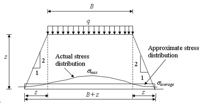
Fig. 6.2. Approximate stress calculation method.

 

Problem 1

Draw the vertical stress distribution due to a concentrated load (Q) of 50 kN acting on the surface of a soil for the following condition by using Boussinesq’s equation:

i) Variation of stress with depth for horizontal distance, r = 0 (points just vertically below the load) and r = 1m.

ii) Variation of stress with horizontal distance (either side of the load) for depth, z = 2m and z = 3m. 

Solution

Equation (6.4) is used to calculate the vertical stress at any depth at any horizontal distance from the point of application of the concentration load. Figure 6.3 shows the variation of vertical stress with depth at horizontal distance, r = 0 and r = 1m. Keeping r value constant, the stress is calculated for different z values upto z = 8m.  For example, at (r = 1m, z = 2m), the vertical stress is 4.22 kN/m².      

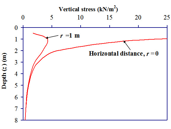
Fig. 6.3. Variation of vertical stress with depth.

Figure 6.4 shows variation of vertical stress with horizontal distance at depth z = 2m and z = 3m. It is observed that as the depth increases vertical stress decreases at the centre line. Same vertical stress is observed at different location with respect to depth and horizontal distance. For example, same vertical stress (2 kN/m²) is observed at (r = ± 1.5m, z = 2m) as well as at (r = ± 1 m, z = 3m). The line joining points with same vertical stress below ground level is called

Isobar.

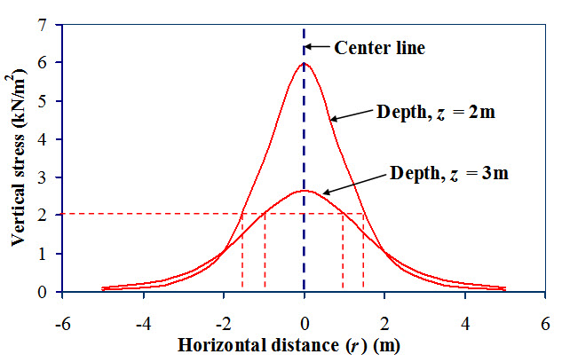
Fig.6.4. Variation of vertical stress with horizontal distance.

 

References

Ranjan, G. and Rao, A.S.R. (2000). Basic and Applied Soil Mechanics. New Age International Publisher, New Delhi, India.

 

Suggested Readings

Ranjan, G. and Rao, A.S.R. (2000) Basic and Applied Soil Mechanics. New Age International Publisher, New Delhi, India.

Arora, K.R. (2003) Soil Mechanics and Foundation Engineering. Standard Publishers Distributors, New Delhi, India.

Murthy V.N.S (1996) A Text Book of Soil Mechanics and Foundation Engineering, UBS Publishers’ Distributors Ltd. New Delhi, India.