Module 1. Conduction heat transfer
Lesson 2
CONDUCTION THROUGH A PLANE WALL
2.1 Conduction through a Plane Homogeneous Wall
Let us consider a plane homogenous wall of thickness “δ” with a constant having thermal conductivity “λ”.
Let us suppose constant
temperature t1 & t2 are maintained on the surface of
walls and temperature varies only in the direction of the x-axis which is
perpendicular to the wall, therefore the temperature field is one dimensional
and the flat isothermal surfaces are arranged perpendicular to the x-axis. Let
us consider inside the wall a layer of thickness dx, located at a
distance “x” from origin outer (surface) and limited by two isothermal
surfaces. Based on Fourier’s law, we can write that ![]() (Specific Rate of heat flow). (Fig. 2.1)
(Specific Rate of heat flow). (Fig. 2.1)
We can solve this differential equation by separating the variables
![]()
![]()
![]()
Where the integration constant “C” can be determined by the boundary condition i.e. when x = 0, t = t1, C = t1
Similarly when we put x = δ, t = t2, therefore we write
![]()
On re-arranging we can write that
![]()
Hence the amount of
heat transferred through 1sqm per hr is directly proportional to thermal
conductivity and the difference in temperature of boundary surface i.e. ∆t
and is inversely proportional to wall thickness “δ”.
This equation is also referred as design formula for conduction through a plane
wall.
-
The
ratio ![]() (kcal/m2-hr-°C)
is known as thermal conductance of the wall and its reciprocal is known as
‘thermal resistance’ of the wall. Thermal resistance is used to determine the
drop in temperature when the rate of heat flow through unit area of wall is
unity.
(kcal/m2-hr-°C)
is known as thermal conductance of the wall and its reciprocal is known as
‘thermal resistance’ of the wall. Thermal resistance is used to determine the
drop in temperature when the rate of heat flow through unit area of wall is
unity.
Now
it is easy to calculate the total amount of heat transferred (Q) through a
plane wall of surface area F (m2) for time τ
(hr)
![]()
Equation of the temperature curve at any location
![]()
The equation of temperature curve is the equation of a straight line. Thus we can say when thermal conductivity is constant, variation in temperature through a homogeneous wall is linear.
When
𝜸
(thermal conductivity) is not constant
Due to the dependence on temperature thermal conductivity is variable for most of the material, this temperature dependence is linear.
![]()
Let us apply Fourier’s law
![]()
![]()
![]()
At x = 0, t = t1,
we get
![]()
At x = δ, t = t2,
we
get
![]()
On
subtraction we get:
![]()
![]()
![]()
This is the specific rate of heat flow through a homogeneous wall when λ is a linear function of temperature:
The equation of temperature curve, that is temperature distribution in the wall, can be obtained by solving the quadratic equation
![]()
Insert the value of C.
Rearrange the quadratic in ‘t’. Then apply the quadratic formula and on solving we get
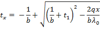
This equation indicates that the temperature inside the wall actually changes along a curved line (Fig. 2.2).
If the factor b is +ve the convexity of the curve faces upward and if b is -ve the convexity of the curve faces downward.
2.2 Conduction through a Composite Plane Wall
Walls of several heterogeneous layers are called composite wall. Also, the wall of dwelling houses in which bricks are covered with a layer of plaster on the inside and on the outside also. Further, the walls of furnace, boiler, cold storages, milk storage tank, vats etc usually are made up of several layers which may include special layer of heat insulation.
Let us derive calculation formula of conduction for composite wall.
Let us assume that the wall consists of 3-hetrogeneous layers. Let us consider walls are in close contact of each other [Fig. 2.3 (a)].
The thicknesses
of the 1st, 2nd and 3rd layer are δ1,
δ2, δ3 respectively. Thermal conductivities of
these layers are λ1, λ2 and
λ3. Let us assume temperature t1
and t4 of outer faces of composite wall are known. Owing to the
perfect contact between the layers, adjacent surfaces have one and the same
temperature. But value of temperature of adjacent layer is not known. Let’s
assume t2 and t3.
Under steady state condition the rate of heat flow per unit area is constant and it is same for all layers. Therefore, we can write.
![]()
![]()
![]()
Rewriting, we get
![]()
![]()
![]()
Adding vertically we get
![]()
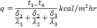
By analogy, the calculations formula for a composite wall of n layers can be written as

Each term in the denominator represent, thermal resistance of respective layer, which mean that total thermal resistance of composite wall is sum of individual resistance. Unknown temperature t2 and t3 can be calculated as:
![]()
![]()
The temperature curve inside each layer is a straight line but for the composite wall it is customary to represent temperature distribution by broken line.
Sometimes to simplify calculation a composite layer is considered a homogeneous plane wall of thickness ∆ and calculations are performed with the aid of the so called ‘Equivalent Thermal Conductivity’
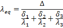
Where ∆
= δ1
+ δ 2 + δ 3
For an n-layer composite wall
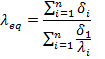
The values Equivalent thermal conductivity depends only on the thermal resistance and thickness of the individual layer. Graphical method for determining intermediate temperatures t2 and t3 is as under: [Fig 2.3 (b)]
of the thermal resistances; ![]() ;
are plotted along the x-axis to any scale, but in order in which layer of the
composite wall are arranged and perpendiculars are erected. Temperatures t1
and t4 are plotted on extreme perpendiculars to an arbitrary
but similar scale. A straight line is plotted by joining t1 and t4.
The points at which this straight line crosses the middle perpendiculars
represents the temperatures t2 and t3.
;
are plotted along the x-axis to any scale, but in order in which layer of the
composite wall are arranged and perpendiculars are erected. Temperatures t1
and t4 are plotted on extreme perpendiculars to an arbitrary
but similar scale. A straight line is plotted by joining t1 and t4.
The points at which this straight line crosses the middle perpendiculars
represents the temperatures t2 and t3.