Module 3. Characteristics of instruments and measurement systems
Lesson 9
dynamic characteristics of measuring instruments
9.1 Dynamic Response
When an input is applied to an instrument or a measurement system, the instrument or the system cannot take up immediately its final steady state position. It goes through a transient state before it finally settles to its final ‘steady state’ position. Some of the measurements are made under such conditions as to allow the sufficient time for the instrument or the measurement system to settle to its final steady state conditions. Under such conditions the study of behaviour of the system under transient state, known as ‘transient response’ is not of much of importance. However, in many areas of measurement systems applications it becomes necessary to study the response of the system under both transient as well as steady state conditions. In many applications, the transient response of the system, i.e., the way system settles down to its final steady state conditions is more important than the steady state response.
The transient response in the instruments is on account of the presence of energy storage elements in the system, such as, electrical inductance and capacitance, mass, fluid and thermal capacitances etc. The systems exhibit a characteristic of sluggishness on account of presence of these elements. However many a times in several applications the measurement systems are subjected to inputs which are not static but dynamic in nature, which means the inputs vary with time. Since the input varies from instant to instant, so does the output. The behaviour of the system under such conditions is described by the dynamic response of the system and the characteristics of the measuring system under such conditions are known as dynamic characteristics.
Dynamic characteristics of a measuring instrument refer to the case where the measured variable changes rapidly. As has been discussed earlier the sensors in control system cannot react to a sudden change in measured variable immediately. A certain amount of time is required before the measuring instrument in control system technology can indicate any output based on the input received by the measuring instrument. The amount of time depends on resistance, capacitance, mass and dead time of the measuring instrument. Step response, ramp response, frequency response of the measuring instrument determines the dynamic characteristics of the measuring instrument in control system technology.
The dynamic characteristics of any measurement system are:
(i) Speed of response and Response time
(ii) Lag
(iii) Fidelity
(iv) Dynamic error
Out of the above four characteristics the Speed of Response and the Fidelity are desirable in a dynamic system, while Lag and Dynamic error are undesirable.
9.2 Speed of Response and Response Time
Speed of Response is defined as the rapidity with which an instrument or measurement system responds to changes in measured quantity.
Response Time is the time required by instrument or system to settle to its final steady position after the application of the input. For a step input function, the response time may be defined as the time taken by the instrument to settle to a specified percentage of the quantity being measured, after the application of the input. This percentage may be 90 to 99 percent depending upon the instrument. For portable instruments it is the time taken by the pointer to come to rest within ±0.3 percent of final scale length and for switch board (panel) type of instruments it is the time taken by the pointer to come to rest within ±1 percent of its final scale length.
9.3 Measuring Lag
As discussed earlier, an instrument does not react to a change in input immediately. The delay in the response of an instrument to a change in the measured quantity is known as measuring lag. Thus it is the retardation delay in the response of a measurement system to changes in the measured quantity. This lag is usually quite small, but this small lag becomes highly important when high speed measurements are required. In the high speed measurement systems, as in dynamic measurements, it becomes essential that the time lag be reduced to minimum.
Measuring lag is of two types
i) Retardation type: In this type of measuring lag the response begins immediately after a change in measured quantity has occurred.
ii) Time delay: In this type of measuring lag the response of the measurement system begins after a dead zone after the application of the input.
9.4 Fidelity
Fidelity of a system is defined as the ability of the system to reproduce the output in the same form as the input. It is the degree to which a measurement system indicates changes in the measured quantity without any dynamic error. Supposing if a linearly varying quantity is applied to a system and if the output is also a linearly varying quantity the system is said to have 100 percent fidelity. Ideally a system should have 100 percent fidelity and the output should appear in the same form as that of input and there is no distortion produced in the signal by the system. In the definition of fidelity any time lag or phase difference between output and input is not included.
9.5 Dynamic Error
The dynamic error is the difference between the true value of the quantity changing with time and the value indicated by the instrument if no static error is assumed.
However, the total dynamic error of the instrument is the combination of its fidelity and the time lag or phase difference between input and output of the system.
9.6 Overshoot
Moving parts of instruments have mass and thus possess inertia. When an input is applied to instruments, the pointer does not immediately come to rest at its steady state (or final deflected) position but goes beyond it or in other words ‘overshoots’ its steady position.
The overshoot is evaluated as the maximum amount by which moving system moves beyond the steady state position. In many instruments, especially galvanometers it is desirable to have a little overshoot but an excessive overshoot is undesirable.
9.6.1 Overshoot
response graph
A typical overshoot response graph can be shown as the response time stated in terms of rise time, peak percentage overshoot and settling time. Such an under damped graph in control system technology of a measuring instrument is shown in Fig. 9.1.
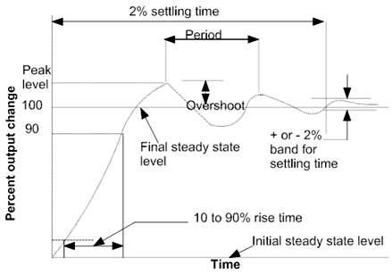
Fig. 9.1 Overshoot response graph
9.6.2 Numerical
1. A step input of 5 A is applied to an ammeter. The pointer swings to a voltage of 5.18 A and finally comes to rest at 5.02 A. (a) Determine the overshoot of the reading in ampere and in percentage of final reading. (b) Determine the percentage error in the instrument.
Solution:
(a) Overshoot = 5.18 – 5.02 = 0.16 A
(b)
![]()
(b) ![]()
9.7 Standard Signals
The measurement systems may be subjected to any type of input. Since in majority of the applications the signals are random in nature and the type of input signals cannot be known ahead of time, it becomes difficult to express the actual input signals mathematically by simple equations. To study the dynamic behaviour of measurement systems, certain standard signals are employed for which the mathematical equations have been developed. These standard signals are:
(i) Step input, (ii) Ramp input, (iii) Parabolic input, and (iv) Impulse input.
The above signals are used for studying dynamic behaviour in the time domain and the dynamic behaviour of the system to any kind of inputs can be predicted by studying its response to one of the standard signals. The standard input chosen for this purpose is a step input.
9.8 Step Response
When the measured variable of a measuring instrument in control system technology encounters changes from one steady state value to a second steady state value it is a step signal and the response shown by the output of a measuring instrument is called the step response. For example, when you change the temperature of the probe of a measuring instrument by shifting it from ice water to boiling water, a sudden temperature change could be observed in the output of the measuring instrument. The step response of such a measuring instrument is stated in terms of response time and rise time for over damped or critically damped situation. Where as for under damped situation the terms used for the measuring instrument are rise time, peak percentage overshoot and setting time. Typical step response curve for an over damped or critically damped measuring instrument is shown in Fig 9.2.

Fig.
9.2 Typical step response curve
Response time is the time required for output to reach a designated percentage of the total change in a measuring instrument. The 95% response time shown in typical step response graph is the time required for output to reach 95% of the total change. 63.2% response time in control system technology of the typical step response graph shown above is the time constant.
9.9 Ramp Response
In the ramp signal the value of signal changes slowly with time. The typical ramp response curve of a temperature measuring instrument is shown in the figure 9.3 below. The measured temperature lagged behind the input temperature, then caught up the input after a certain period of time. This figure allows us to view two response curves, the dynamic error and dynamic lag.
Fig.
9.3 Typical ramp response curve
Dynamic lag of a measuring instrument is the amount of time that passes between the time the input reaches a certain temperature and the output that follows input reaches also at the same temperature. A horizontal line at T1 on the dynamic response graph intersects with input curve at time t1 and the output curve at time t2. The difference between these two times is defined as the dynamic lag at temperature T1.
Dynamic error of a measuring instrument is the difference between input temperature and output temperature at a given time. It is the vertical line at a time t2 on the ramp response graph that intersects the output curve at temperature T1 and the input curve at temperature T2. The difference between these two temperatures is the dynamic error at time t2.