Module 6. Process control

Lesson 27

ELEMENTS OF GENERALIZED PROCESS CONTROL

27.1  Introduction

Most industrial processes require that certain variables such as temperature, flow, level or pressure and concentration, remain at or near some reference value (set-point). The set-point is a value for a process variable that is desired to be maintained. A closed control loop exists where a process variable is measured, compared with a set-point and action is taken to correct any deviation from the set-point. The system that serves to maintain a process variable at the set point is called controller which is the part of a control system. In automatic control system, controller performs the basic operation used by many systems provides regulation or command to the process variable to be controlled. Our goal using this type of feedback control is to determine the value or state of some physical quantity and often to maintain it at that value, despite variations in the system or the environment.

Automatic control system provides the means of attaining optimal performance of dynamic systems and improving productivity. This defines as a series of operations during which some materials are placed in more useful state by continually measuring process variables (A process variable is a condition of the process fluid that can change the manufacturing process in some way) and taking actions such as opening valves, slowing down pumps and turning up heaters so that the measured process variables are maintained at operator specified set point values. Mainly there are four basic objectives of automatic process control which are as under.

1. Suppressing the influence of external disturbances

2. Optimizing the performance

3. Increasing the productivity

4. Cost effective

27.2  Fundamental Structure of Control Systems

A control system is that means by which any quantity of interest in a machine or mechanism can be changed, maintained or unaltered in accordance with desired manner. This system uses an interconnection of components forming a system configuration that will provide a desired system response. Input Signals flow through the system and produce an output as shown in Fig.27.1(a).

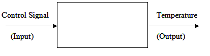
Fig. 27.1 (a) Representation of input and output of a process

The input will usually be an ideal form of the output.  In other words the input is really what we want the output to be.  It's the desired output. The output of the system has to be measured.  In the Fig. 27.1 (b), we have shown the system in which we are trying to control - the "plant" and a sensor that measures what the controlled system is doing.

The input to the plant is usually called the control effort, and the output of the sensor is usually called the measured output, as shown Fig. 27.1 (b).

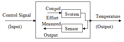
Fig. 27.1 (b) Representation of input and output of a process

For example, if we want the output to be 100°C, then that's the input.

To control the process output, it is necessary to first measure the process output which is to be controlled at a desired set point. The sensor measures the actual process output. In the block diagram representation (Fig. 27.2), the sensor senses the process-output temperature and generates a proportionate output signal. A sensor might be an LM35, which produces a voltage proportional to temperature - if the output signal is a temperature. Sensor is needed in the system to measure what the system is doing. The sensor measures the output e.g. temperature of the system to be controlled, and converts it into proportionate electrical signal. The LM35 temperature sensors, for example, produce 0.01 volts for every 1.0°C change. To control the system we need to use the information provided by the sensor. Usually, the output, as measured by the sensor is subtracted from the input (which is the desired output) as shown in Fig. 27.2. That forms an error signal that the controller can use to control the plant.

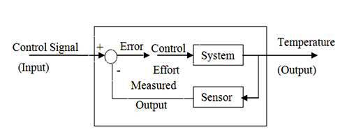
Fig. 27.2 Representation of input and output of a process with error comparator

The device which performs the subtraction to compute the error E is a comparator. Finally, the last part of this system is the controller which is as shown in Fig.27.3.

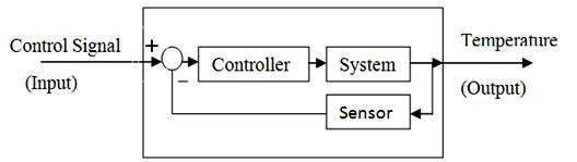
Fig. 27.3 Block diagram of negative feedback control loop

The controller receives the error signal from the comparator and generates an actuating signal which can be used to control the process-output through the actuating element. Thus, the controller has two functions:

1. To compute what the control effort should be.

2. To apply the computed control effort.

27.3  Types of Control System

Mainly there are two types of control system:

1) Open-loop systems and

2) Closed-loop systems

27.3.1  Open loop systems

The open-loop system (Fig. 27.4) is also called the non-feedback system. It utilizes an actuating device to control the process directly without using feedback. Gas geyser, electric geyser etc. used for heating of water are few examples of open-loop control system. This is the simpler of the two systems. However, since it is not possible to achieve desired accuracy of control of the parameter and its use is limited in the industry. In open- loop control system there is only a forward action from the input to the output.

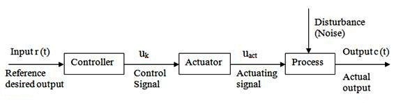
Fig. 27.4 Block diagram of open-loop control system

27.3.2  Closed loop systems

The closed-loop system is also called the feedback system. Feedback control system is to control the process by using the difference between the output and reference input. A closed-loop control system uses a measurement of the output and feedback of this signal to compare it with the desired output (reference or command) as explained above in Section 27.2.

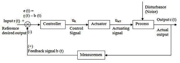
Fig. 27.5 Block diagram of closed-loop system

The basic functions of an automatic controller in a closed-loop system are:

1) To receive the actual measured value of the variable being measured.

2) To compare that value with a reference or desired value.   

3) To determine the deviation with the help of comparator.

4) To provide an output control signal to reduce the deviation to zero or a small value.

27.4  Basic Elements of Generalized Process Control

In the process control, four basic elements are normally involved:

1. Process

2. Measurement

3. Evaluation (with a controller)

4. Control element

Fig. 27.6 shows the block diagram of generalized process control and the function of each block are given as follows:

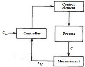
Fig. 27.6 Block diagram of generalized process control

1. Process

The term Process as used in relation to process control refers to the methods of converting raw materials into the end product(s). The raw materials which either pass through or remain in a liquid, gaseous, or slurry (a mix of solids and liquids) state during the process, are transferred, measured, mixed, heated or cooled, filtered, stored, or handled in some other way to produce the end product. Many dynamic variables may be involved in a process, and it may be desirable to control all these variables at the same time. There are single-variable processes, in which only one variable is to be controlled. However, most industrial processes are multivariable processes, in which many variables, perhaps interrelated, may require regulation.

2. Measurement

To perform control, it is necessary to measure the process parameter, so that we can have information on the variable itself. In general, a measurement refers to the transduction of the variable into some corresponding analog of the variable, such as a pneumatic pressure, an electrical voltage, or current. A transducer is a device that performs the initial measurement and energy conversion of a dynamic variable into analogous electrical or pneumatic information. Further transformation or signal conditioning may be required to complete the measurement function. The result of the measurement is a transformation of the dynamic variable into some proportional information in a useful form required by the other elements in the process-control loop.

3. Evaluation

The next step in the process-control sequence is to examine the measurement and determine what action, if any, should be taken. The evaluation may be performed by an operator, or by electronic/pneumatic signal processing, or by a computer. A controller is a device that receives data from a measurement instrument, compares that data to a programmed set-point, and, if necessary, signals a control element to take corrective action. Computer use is growing rapidly in the field of process control because it is easily adapted to the decision making operations and because of its inherent capacity to handle control of multivariable systems. The controller requires an input of both a measured representation of the dynamic variable and a representation of the desired value of the variable, expressed in the same terms as the measured value. The desired value of the dynamic variable is referred to as the set point. Thus, the evaluation consists of a comparison of the controlled variable measurement and the set point and a determination of action required to bring the controlled variable to the set point value.

4. Control element

The correcting or final control element is the part of the control system that acts to physically change the manipulated variable. This element accepts an input from the controller, which is then transformed into some proportional operation performed on the process. In any process control loop, final control elements are typically used to correct a variable that is out of set-point.

In most cases, the final control element is a valve/servo motor used to restrict or cut off fluid flow, but motors, louvers (typically used to regulate air flow), solenoids, and other devices can also be final control elements. For example, a final control element may regulate the flow of fuel/air to a burner to control temperature, the flow of a catalyst into a reactor to control a chemical reaction.

A block diagram can be used simply to represent the composition and interconnection of a system. Also, it can be used together with transfer function to represent the cause and effect relationship throughout the system. Transfer Function defines the relationship between an input signal and an output signal for a system.

Each element in a process-control loop is represented in a block diagram as a separate step. The controlled dynamic variable in the process is denoted by C and the measured dynamic variable is labeled as C_M. The controlled variable set point, labeled C_SP, must be expressed in the same proportion as that provided by the measurement function. The evaluation operation generates an error signal (E = C_M - C_SP) to the controller for comparison and corrective action.

To further illustrate, the block diagram concept in Fig. 27.7 shows a typical flow control system. In this example, the dynamic variable is the flow rate that is converted to electric signal as an analog. The process is the flow, and the measurement is to determine the difference of pressure. With the set point in the controller, the flow of the process is controlled through the control element i.e. the valve.

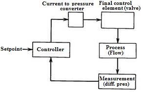
Fig. 27.7 Process Control System to regulate flow and the corresponding block diagram

27.5  Process Equations

The purpose of a process control loop is to regulate some dynamic variable in a process. The dynamic variable or a process parameter may depend on many other parameters (in the process) and thus suffer changes from many different inputs. One of these parameters is selected as a controlling parameter. This means that if a measurement of variable shows the deviation from the set point, then the controlling parameter is changed. For an example, consider the control of liquid temperature in tank shown in Fig. 27.8.

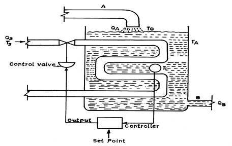
Fig. 27.8 Hot water temperature control system

Here the dynamic variable is the liquid temperature T_L. This temperature depends on many  parameters in process like input flow rates in pipe A, output flow rates via pipe B, ambient Temperature T_A, the steam temperature Ts, inlet temperature To, and the steam flow rates Q_S. In this case, steam flow rate is the controlling parameter. If one of other parameters changes, accordingly there is change in temperature results. In order to bring the temperature back to the original value the steam flow rate is adjusted accordingly. This can be described by a process equation where liquid temperature is a function as:

T_L = F (Q_A, Q_B, Q_S, T_A, T_S, T_B, T_O)

Where:

Q_A, Q_B = flow rates in pipes A and B

Q_S = Steam Flow rate

T_A = ambient temperature

T_O = Inlet fluid temperature

T_S = steam temperature

27.5.1  Process load

Process load refers to set of all parameters excluding the dynamic variable. At some point in time, a process load change causes a change in dynamic variable e.g. when all parameters in a process have their nominal values, it is known as the nominal load on the system. The required control parameters value under these conditions is the nominal value of that parameter. If the set point is changed, then the control parameter is altered to cause the variable to adopt new operating point. The load is still nominal, however, because of other parameters are assumed unchanged. Now if one of the parameters changes from nominal value, causing a corresponding shift in the controlled variable then a process load change is said to have occurred.

27.5.2  Process lag

It represents a delay in reaction of controlled variable to a change of load variable e.g. the process control loop in a process responds to assure, some finite time later that the variable returns to set point value. Part of this time is consumed by the process itself and referred to as process lag. Process time lags are affected by capacitance which is the ability of a process to  store  energy;  resistance,  the  part  of  the  process  that  opposes  the  transfer  of energy between capacities and transportation time, the time required to carry a change in a process variable from one point to another in the process. This time lag  is  not  just  a  slowing  down  of  a  change,  but  rather  the  actual  time  delay during which no change occurs.

27.5.3  Self-regulation

Self regulation is characteristic that a dynamic variable adopts some nominal value commensurate with the load with no control action. The output will move from one steady state to another for the sustained change in input. This means that for change in some input variable the output variable will rise until it reaches a steady state (inflow = outflow). It is the tendency of the process to adopt a specific value of controlled variable for nominal load with no control operations. A significant process characteristic is its tendency to find a specific value of dynamic variable for nominal load with no control operations. The control operations may be significantly affected by such self-regulation. The process of Fig. 27.8 has self regulation as shown by the following arguments:

(a) Suppose we fix the steam valve at 50 % and open the control loop so that no changes in valve position are possible.

(b) The liquid heats up until the energy carried away by the liquid equals that input energy from the steam flow.

(c) If load changes, a new temperature is adopted (because the system temperature is not controlled).

(d) The process is self regulating because the temperature will not run away but stabilizes.