Module 1. Alternating and direct current: Fundamentals

Lesson 5

PHASE RELATIONS AND VECTOR REPRESENTATION

5.1  Introduction

Sinusoidal varying alternating quantity (Current or Voltage) may be represented in following three ways:

a. Graphically represented by wave form.

b. Mathematical equation of instantaneous value of an alternate quantity.

c. Phasor Diagram: Phasor is a line of definite length to represent an alternating quantity. The length of this line is equal to the maximum value of the alternating quantity. It rotates in anti-clockwise direction at angular velocity ω radians/ second.

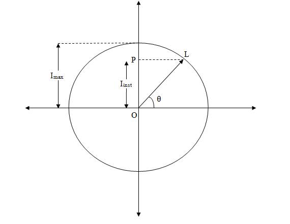
Fig. 5.1 Phasor for alternating current

Let us consider an alternating current i = I_max Sin ωt. The phasor is shown in fig. 5.1.

· The phasor OL rotating in anti-clockwise direction is representing the alternate current.

· The horizontal dotted projecting phasor OP on Y-axis gives the value of the current at that instant (I_inst).

· The lengthy phasor (i.e OL) gives the maximum value of current, I_max..

· The angle of the phasor with the horizontal x-axis represent the angle of the alternating current θ. This angle θ is also known as phase of the alternating quantity.

· I is the value of current at that instance and is given by equation:

i = i_max Sin ωt   (Where θ = ωt)

· The angular velocity of phasor is ω radian/ sec about point O.

5.2  Phasor Diagram of Similar Alternating Quantity

Let us consider two alternating currents of same frequency of magnitude I_m1 and I_m2. Two alternating quantities having same frequency but having different zero points are said to have a phase difference.

As shown in figure 5.2, the angle between the zero points of two alternating current is called phase angle or angle of phase difference ϕ. Phase angle can be measured as degrees or radians.

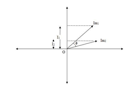
Fig. 5.2 Phasor Diagram of similar alternating quantity

5.2.1  The concept of leading and lagging

Alternating quantities with different zero points have a phase difference generally measured as angle ϕ.

Leading: The quantity which attains zero point earlier than the other quantity is known as leading quantity.

Lagging: The quantity which attains zero point later than the leading quantity is known as lagging quantity.

In figure 5.2 I₁ is the leading current w.r.t I₂, And I₂ is the lagging current w.r.t. I₁. The phase difference between them is ϕ.

5.3  Phasor Diagram of Different Alternating Quantity

In case of two alternating quantities e.g. current & voltage, let us consider following assumptions:

1. Two alternating quantities voltage V and current I of same frequency.

2. Voltage is leading w.r.t current by phase difference of ϕ angle.

3. These alternating quantities can be shown by phasor diagram (Fig. 5.3).

4. The phasor V_m and I_m rotate at the same angular velocity ω radian / sec.

5. Due to same angular velocity the phase difference ϕ between two phasors V_m and I_m remains constant.

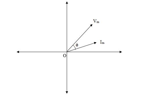
Fig. 5.3 Phase difference ϕ between two phasors V_m and I_m

5.4  Addition and Subtraction of Alternating Quantities

5.4.1  Addition of alternating quantities

There are certain rules for addition of alternating quantities:

a) Alternating quantities like voltage and currents can be represented as phasor.

b) These phasor can be added in the same manner as forces are added.

c) Only alternating quantities of similar types can be added. Either voltages can be added or currents can be added. Voltage cannot be added to current.

Alternating voltage or current can be added by any of the following methods:

i. Parallelogram method.

ii. Method of components.

5.4.1.1  Parallelogram method

This technique is used for addition of two phasors at a time. The two alternating quantities are denoted by phasor diagram. The two phasors are arranged as the adjacent sides of a parallelogram. The diagonal of the formal parallelogram gives the resultant value of the two phasors. The following diagram shows phasor diagram of a.c parallel circuit:

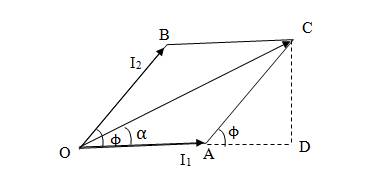
Fig 5.4 Phasor diagram of a.c parallel circuit

The two currents flowing in the circuit are given as:

i₁= I_m1Sin ωt

i₂= I_m2 Sin (ωt +ϕ)

i_r= resultant current

I_m1 and I_m2 are the maximum value of currents i₁ and i₂ respectively. Here i₁ is leading w.r.t i₂ or in other words i₂ is lagging w.r.t i₁. The phase difference between i₁ and i₂ is ϕ^o.

The equation for instantaneous value of resultant current i_r is given as:

i_r = I_mr Sin (ωt + α)

5.4.1.2  Method of components

This method can be used to add two or more phasors. The steps are as follows:

· Draw the phasor diagram for each alternating quantity.

· Resolve each phasor into horizontal and vertical components.

· Add all the horizontal components algebraically to obtain the resultant horizontal component I_x.

· The entire vertical component algebraically to obtain the resultant vertical component I_y.

· The resultant value of the alternating quantity will be calculated as:

5.5  Subtraction of Alternating Quantities

The steps for subtraction of alternating quantities are described below:

1. Draw phasor diagram for the two alternating quantities.

2.  One of the phasor is traced and drawn in reverse direction.

3.  Now it can be solved by parallelogram method or method of component.

Two similar alternating quantities i.e current i₁ and i₂ is given by phasor OA and OB.

The subtraction can be given by = OA –OB

= phasor OC