Module 3. Characteristics of instruments and measurement systems
Lesson 7
Static characteristics of measuring instruments - II
7.1 Scale Readability
This indicates the closeness to with which the scale of an analog type of instrument can be read. The readability of an instrument depends upon following factors:
i) Number of graduations
ii) Spacing between the graduations
iii) Size of the pointer
iv) Discriminating power of the observer
The readability is actually the number of significant figures in the instrument scale. The higher the number of significant figures, the better would be the readability.
7.2 Repeatability and Reproducibility
Repeatability is the degree of closeness with which a given value may be repeatedly measured. It is the closeness of output readings when the same input is applied repetitively over a short period of time. The measurement is made on the same instrument, at the same location, by the same observer and under the same measurement conditions. It may be specified in terms of units for a given period of time. Reproducibility relates to the closeness of output readings for the same input when there are changes in the method of measurement, observer, measuring instrument location, conditions of use and time of measurement. Perfect reproducibility means that the instrument has no drift. Drift means that with a given input the measured values vary with time.
Reproducibility and Repeatability are a measure of closeness with which a given input may be measured over and over again. The two terms cause confusion. Therefore, a distinction is made between the two terms. Reproducibility is specified in terms of scale readings over a given period of time. On the other hand, Repeatability is defined as the variation of scale reading and is random in nature.
7.3 Drift
Drift is a departure in the output of the instrument over the period of time. An instrument is said to have no drift if it produces same reading at different times for the same variation in the measured variable. Drift is unrelated to the operating conditions or load. The following factors could contribute towards the drift in the instruments:
i) Wear and tear
ii) Mechanical vibrations
iii) Stresses developed in the parts of the instrument
iv) Temperature variations
v) Stray electric and magnetic fields
vi) Thermal emf
Drift can occur in the flow meters due to wear of nozzle or venturi. It may occur in the resistance thermometer due to metal contamination etc.
Drift may be of any of the following types;
a) Zero drift: Drift is called zero drift if the whole of instrument calibration shifts over by the same amount. It may be due to shifting of pointer or permanent set.
b) Span drift: If the calibration from zero upwards changes proportionately it is called span drift. It may be due to the change in spring gradient.
c) Zonal drift: When the drift occurs only over a portion of the span of the instrument it is called zonal drift.
Drift is an undesirable quality in industrial instruments because it is rarely apparent and cannot be easily compensated for. Thus, it must be carefully guarded against by continuous fields can be prevented from affecting the measurements for proper shielding. Effect of mechanical vibrations can be minimized by having proper mountings. Temperature changes during the measurement process should be preferably avoided or otherwise be properly compensated for.
7.4 Static Sensitivity
The static sensitivity of an instrument or an instrumentation system is the ratio of the magnitude of the output signal or response to the magnitude of input signal of the quantity bring measured. Its units depend upon the type of input and output. If the output is in mm and the input is in micro ampere then the units would be mm per micro-ampere.
Sometimes the static sensitivity is also expressed as the ratio of the magnitude of the measured quantity to the magnitude of the response. Thus the sensitivity expressed this way has the units of micro-ampere per mm. It is reciprocal of the sensitivity as defined above. This ratio is defined as the inverse sensitivity or defection factor. Many manufacturers define the sensitivity of their instruments in terms of inverse sensitivity and still call it sensitivity.
The sensitivity is expressed as the slope of the calibration curve if the ordinates are expressed in actual units. When a calibration curve is linear the slope of the calibration curve is constant. For this case the sensitivity is constant over the entire range of the instrument. However, if the curve is not a straight line, the sensitivity varies with the input.
In general, the static sensitivity at the operating point is defined as:
![]()
Similarly,
![]()
The sensitivity of an instrument should be high and therefore the instrument should not have a range greatly exceeding the value to be measured. However, some margin should be kept for any accidental overloads.
7.5 Numericals
1. A pressure gauge which has a linear calibration curve has a radius of scale line as 120 mm and pressure of 0 to 50 Pascal is displayed over an arc of 300o. Determine the sensitivity of the gauge as a ratio of scale length to pressure.
Solution:
![]()
![]()
![]()
![]()
2. A Wheatstone bridge requires a change of 7.000 Ω is the unknown arm of the bridge to produce a change in deflection of 3.000 mm of the galvanometer. Determine the sensitivity. Also determine the deflection factor.
Solution:
![]()
It may be noted that
i) A sensitive instrument can quickly detect a small change in measurement.
ii) Measuring instruments that have smaller scale parts are more sensitive.
iii) Sensitive instruments need not necessarily be accurate.
7.6 Linearity
When the input-output points of the instrument are plotted on the calibration curve and resulting curve may not be linear. This would be only if the output is proportional to input. Linearity is the measure of maximum deviation of these points from the straight line (Fig. 7.1). The departure from the straight line relationship is non-linearity, but it is expressed as linearity of the instrument. This departure from the straight line could be due to non-linear elements in the measuring system or the elastic after effects of the mechanical system.
Linearity is expressed in many different ways:
i) Independent Linearity: It is the maximum deviation from the straight line so placed as to minimize the maximum deviation (Fig. 7.1).
ii) Zero based linearity: It is the maximum deviation from the straight line joining the origin and so placed as to minimize the maximum deviation.
iii) Terminal based linearity: It is the maximum deviation from the straight line joining both the end points of the curve.
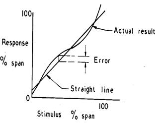
Fig. 7.1 Independent linearity
Linearity of out-input relation is considered to be one of the best characteristics of the measurement system, because of the convenience of scale reading. The non linear relation does not lead to any inaccuracy, but it is better to keep the linearity as small as possible, by choosing the operating range instrument in such a way that the input-output relation is linear. Lack of linearity thus does not necessarily degrade sensor performance. If the nonlinearity can be modelled and an appropriate correction applied to the measurement before it is used for monitoring and control, the effect of the non-linearity can be eliminated.
7.7 Dead Band and Dead Time
Dead band, sometimes called a neutral zone, is an area of a signal range or band where no action occurs, that is, the system is dead e.g. 10 g weight on a 10 kg balance. It is the largest change in the physical variable to which the measuring instrument does not respond. In other words it is defined as the range of input values over which there is no change in output value. It has also been referred to as Dead space or Dead zone. In the analog instruments, it may occur due to friction in the instrument which does not allow pointer to move till sufficient force is developed to overcome the frictional loss. It is shown in the figure 7.2.
Fig. 7.2 Dead band or dead space of measuring instruments
Dead zone is specified by indicating it as the percent of span range. For example, if the calibration range of a thermometer is 100 to 300°C and the dead zone is specified as 0.1% of the span, then the change in temperature that must occur before it is detected by the instrument would be:
(300 -100) x 0.1 / 100 = 0.2°C
Dead band is different from hysteresis. Dead band is purposefully used in voltage regulators and other controllers to prevent oscillation or repeated activation-deactivation cycles.
Dead time is the time required by measuring instrument to begin to respond to a change in the measured variable. It represents the time before the instrument begins to respond after the measured variable has changed. The units of dead zone are the units of the variable, whereas, the units of the Dead time are the units of time.