Module 4. Database systems
Lesson 9
DATABASE STRUCTURES
9.1 Introduction
Students will learn about the concept of data association, entity relationship diagram, Hierarchical (tree), Network (plex), and relational database models. These topics will be useful for students to understand the concept natural association among the data values and different types of database models.
9.2 Data Associations
Data items by themselves do not convey any meaning. For example, a given set of value of dairy plants and another of products supplied by the plants as in the following table 9.1, does not communicate anything:
Table 9.1 Dairy plants and products supplied
|
Dairy Plants |
Product Supplied |
|
Mother Dairy, Delhi |
Dairy Whitener |
|
NDRI, Karnal |
Ghee |
|
Parag, Gaziabad |
Ice-cream |
|
Nestle, Moga |
Tonned Milk |
However, if it is informed that the dairy plant, Mother dairy manufactures Ice-cream, NDRI manufactures Ghee, Nestle manufactures dairy whitener etc., immediately conveys some information. This information is available because a data association has been established between the values of Dairy plants and the product supplied by them. Data association is a correspondence or mapping between the members of two sets, e.g. the correspondence, in above table between Dairy plants and products supplied is given by writing them on the same line. The data association between the data items is also known as relationship or mapping. Schema and subschema are maps showing the data item types and relationships between them. The data association exists at two levels in database 1) between two or more data items i.e. attributes and 2) between two or more records (entities) / tables. There are various ways of drawing the associations.
The association between two data items (attributes) can be of two types as described below:
9.2.1 One-to-one (1 : 1)
In this type of association there is one-to-one mapping from data item A to data item B. This means that each value of A has one and only one value of B associated with it. For example Product name and its code have one to one relationship, an employee ID number, and his GPF number have 1:1 correspondence. This type of relationship is shown in fig. 9.1 by single arrow.
![]()
Fig. 9.1 One-to-one data association
9.2.2 One-to-many (1 : M)
In this type of association there is one-to-many mapping from data item A to data item B. This means that one value of A has one or more values of B associated with it. For example on a particular route there may be more than two or more societies for collection of milk, parent and child relationship have 1:M correspondence. This relationship is shown in fig. 9.2 by double arrow.
![]()
Fig. 9.2 One-to-many data association
A one-to-one association is also referred as simple and one-to-many association as complex mapping. Mapping between two data items is always in both directions thus there may be four combination of associations in forward and reverse directions such as 1:1, 1:M, M:1, M:M. In M:M type of relationship there is many-to-many mapping from data item A to data item B and vice versa. This means that one value of A has one or more value of B associated with it and similarly one value of B has one or more value of A associated with it. For example one product may be packed in different packaging sizes and one packaging size may be used for packing different products, a vendor may supply many products as well as a product may be supplied by many vendors. This relationship is shown in fig. 9.3 by double arrow at both ends.
![]()
Fig. 9.3 Many-to-many data association
In addition to these associations there is another type of association which is distinguished as conditional mapping or relationship from A to B. This means that each value of A may have one or zero values of B associated with it. For example milk received in the plant may or may not be sanctioned for manufacturing sweats on particular day.
The association between two records (entities) can be of same types as described above say 1:1, 1:M, M:1, M:M and conditional relationship. As discussed in previous chapter a record is a collection of related attributes. Record is uniquely identified by an attribute known as primary key. For example the details of milk can be grouped as one record containing date of milk receipt, society number, route number, time of milk collection, type of milk, quantity of milk, fat%, SNF%, pH, acidity, etc. Graphically a record is drawn as an elongated box with number of attributes. Primary key of the record is distinguished from other attributes by underlining it. Primary key may be a combination of more than one attributes. Milk details record is identified by a key which is a combination of attributes i.e. ReceiptDate + SocietyNo + MilkTime + MilkType. Similarly details of routes, societies, different sections in a dairy plant, details of milk manufactured, sale details of milk products etc. may be grouped in different records. The relationship between society and milk details is 1:M since one society may have many records in milk details record (one record for each time of milking) and may be depicted as shown in fig. 9.4 given below:

Fig. 9.4 One-to-many data association between records
9.2.3 Procedure for drawing a schema using data association
I. Collect all data items (attributes) and group them into records clearly.
II. Each attribute is given a short name as well as record for reference.
III. The diagram should clearly distinguish between the names of data items and records
IV. Record name is written outside on top and attributes name inside the box.
V. Duplicate name should not be used.
VI. Primary key should be made clear.
VII. Where secondary keys are an important part of the schema, these should be made clear (for example by drawing double arrow headed line from secondary key to primary key of the record)
VIII. Data association should be clearly depicted in the diagram using arrow lines.
IX. If associations between records are given names these should be on the diagram.
Example-1: Consider the HRD department name of a dairy plant where all details pertaining to employees of the plants are being maintained, e.g., Employee ID, name, date of birth, salary, department, skill, number of children etc. All this information may be grouped into different records and the relationship between records as shown in figure 9.5 given below. Relationship from EMPLOYEE to SKILL and CHILD is one sided i.e. only downward link 1:M is shown not the upward link, i.e., not from SKILL to EMPLOYEE and CHILD to EMPLOYEE since for these, this path is not intended to be Sused.

Fig. 9.5 One of drawing schema for employees
Example-2: Consider another example of purchasing items in the store of a plant. Generally a list of items being used in the plant is maintained as well as list of suppliers. Whenever an item is to purchased quotations are invited from the supplier for the item to be purchased. The purchase order is placed with the supplier who is fulfilling the quality constraints and has quoted the lowest rate. Schema for this kind of problem is shown in fig. 9.6.
Example-3: Consider the schema described in fig. 9.5. For users working in account section and users working in HRD and training section may have different sub schemas as per their own requirement as shown in fig. 9.7 (a) and 9.7 (b) respectively given below.
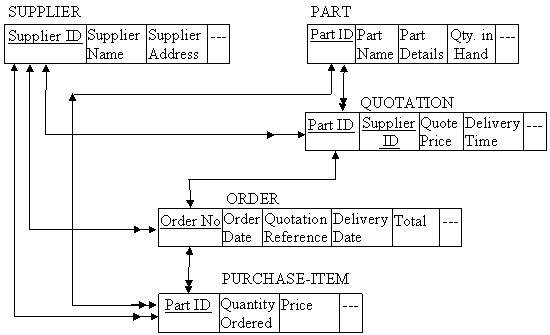
Fig. 9.6 Schema for purchase orders
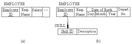
Fig. 9.7 Subschema for (a) account section and (b) HRD and training section
9.3 Entity Relation Model and Diagram
Entity-Relationship (ER) model is a conceptual data model that views the real world as entities and relationship. A basic component of the model is Entity Relationship diagram which is used to visually represent data objects. This model was originally introduced by Peter in 1976 as a way to unify the network and relational database views. Since its origin the model has been extended and is being commonly used for database design by database administrators. It maps the relationship among data items very simply and naturally. ER model can be used as a design plan by database developers to implement a data model in a specific DBMS. The constructs used in ER diagram can easily be transformed into database structure.
9.3.1 Basic components of ER diagram
The ER diagram views the real world situation in form of entities and association between entities. So, let us first understand few important components used in ER diagram:
I.
Entities:
Entities are usually recognizable
concepts either concrete or abstract such as persons, places, things, or events
which have relevance to the database. Some specific examples of entities are employees,
milk products, manufacturing losses, milk societies etc. An entity set is a
set of entities of same type that share the same properties, e.g., set of all
employees, dairy plants etc.
II.
Independent
entities: The
entities that do not rely on others for identification.
III.
Dependent
entities: The
entities that rely on others for identification.
IV.
Associative
entities: These
entities are used to associate two or more entities in order to reconcile a M:M
relationship and also known as intersection entities.
V.
Relationships:
Relationships represent an
association between two or more entities. These provide the structure needed to
draw information from multiple entities.
VI.
Degree
of a relationship: The
number of entities associated with the relationship. The n-ary is the general
form of representing the relationship of degree n e.g. binary -between 2
entities, ternary – among 3 entities etc.
VII.
Connectivity:
It describes the mapping of
associated entities instances in the relationship. There are three types of
connectivity 1. One-to-One, 2. One-to-Many, 3. Many-to-Many.
VIII.
Cardinality:
Cardinality of a relationship is the
number of related occurrences for each of the two entities.
9.3.2 Symbols used in ER diagram
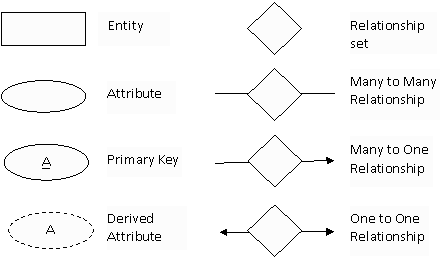
Information in ER diagrams is represented with the help of symbols. Three basic symbols used are Entity, attribute and Relationship. Other are derived from these symbols. There is no standard for representing data objects in ER diagrams. Each modeling methodology uses its own notation. However Scommonly used symbols or notations for drawing ER diagram are described in fig. 9.8 given below.
Fig. 9.8 Symbols used in ER diagram
9.3.3 Example for developing ER diagram
Developing an ER diagram requires an understanding of the system and its components. Before discussing the procedure, let's look at the example narrated as follows:
Consider the milk procurement activity in brief:
· Milk procurement area is identified.
· Societies are created in each village. These societies are managed by villagers.
· Milk producers/ Farmers become members of the societies.
· Quality of milk is checked at the time of taking milk from the members. Members contribute milk in morning and evening time.
· Optimized routes are designed by plant to collect milk from societies. Vehicle is sent to all societies to collect milk.
· Milk is delivered to the dockyard of the dairy plant at both times or one time as per the policy of plant. Again milk quality is checked at the dockyard.
· Payment is made to farmers based on the quality of milk as per the policy of plant (weekly/ fortnightly/ 10 Days etc.)
9.3.4 Steps for drawing ER diagram
Following steps are involved in planning and drawing the ER diagram:
I. Define Entities: These are usually nouns used in descriptions of the system, in the discussion of business rules, or in documentation; identified in the narrative (see highlighted/ bold items above).
II. Define Relationships: These are usually verbs used in descriptions of the system or in discussion of the business rules (entity to entity); identified in the narrative (see bold italic items above).
III. Add attributes to the relations and entities: these are determined by the queries, and may also suggest new entities. List of attributes are decided based on the purpose of creation of database or the problem to be solved.
IV. Add cardinality to the relations: Many-to-Many relationship must be resolved to one-to-many relationship with an additional entity called associative entities. Usually this happens automatically but sometimes involves introduction of a link entity (which will be all foreign key) Examples: Route-Vehicle information.
For the above problem ER diagram may be drawn as shown in fig. 9.9 given below.
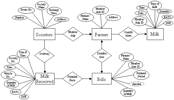
Fig. 9.9 ER diagram for milk procurement activity
9.4 Database Models
A database model provides theoretical foundation for developing a database and basically determines how data can be stored, organized, retrieved, updated and manipulated in a database system. It represents the collection of conceptual tools for describing data, relationships, semantics, operations that are performed on data and data constraints. It describes the idea of a complex “real-world” data structure. A database model contains structural, manipulative and data integrity parts. Based on the organization and relationship of data items related to different entities in real world, database models may be grouped as follows:
· Record-based models: In this model, real world entities are represented in form records. Each record has a fixed number of attributes (also known as fields) and each field has a fixed data type and size usually for easy implementation. Thus record-based database is structured in fixed format records of various types. The three most widely accepted models are hierarchical (tree), network (plex) and relational models.
· Object-based models: These are the models that are most popular in designing the database. These models involve object oriented concepts for designing the database.
· Physical models: Physical database models describe data at lowest level for storage on devices. Very few models are available for this purpose, e.g., Unifying model, Frame memory etc.
9.5 Hierarchical Model
Hierarchical data model organizes data in a tree-like structure. There is a hierarchy of parent and child relationship. All attributes and instances of an entity are listed in form of a table (or record type or entity type) in database. Columns of table are known as fields and rows representing instances of entity are called as records. Hierarchical model uses Parent-Child relationship to create links between these tables (or record type) i.e. 1: M mapping between record types. Hierarchical structures were widely used in the first mainframe database management systems. However owing to their restrictions, they often cannot be used to relate structure that exists in real world. Hierarchical relationship between different types of data can make it very easy to answer some questions, but very difficult to answer others. Hierarchical DBMSs were popular from the late 1960s to 1970s with the introduction of IBM's Information Management System (IMS) DBMS.
Hierarchical model is based on tree structure. A tree is composed of a hierarchy of elements called node, the uppermost level of the hierarchy has only one node, called the root. Except the root node, every node has one node related to it at a higher level called as parent node. No element can have more than one parent. Each element can have one or more elements related to it at a lower level. These are called children. Elements at the end of the branches are called leaves. A tree can be defined as a hierarchy of nodes with binodal relationships such that:
- The highest level in the
hierarchy has one node called a root.
- All nodes except the root are only one node on a higher
level than themselves.
Fig. 9.10 shows a tree structure with 19 elements (nodes) where element 1 is root node and elements 5, 14 and 19 as leaves. Trees are normally drawn upside down with root at top and leaves at bottom. There are four levels in this tree, level 1 represent root, level 2, 3 and 4 represent branches. Trees are used in both logical and physical data descriptions. In logical description these are used to describe relations between tables/ entity type/ record type while in physical description these are used to describe sets of pointers and relations between physical segments of data values.
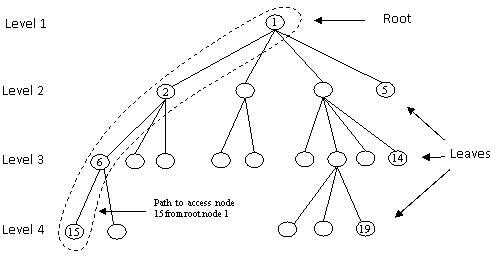
Fig. 9.10 A tree structure
9.5.1 Hierarchical files
This refers to a file with a tree structure relationship between the records. Data tend to break down into hierarchical categories. One category of data is a subset of another. A record may have multiple records subordinate to it, which in turn may have multiple records subordinate to them. In other words, multiple records of a particular type belong to (or subordinate to) a single record of another type higher in the hierarchy. For example in inventory of finished milk products the relationship between Master record type of product and transaction record type of product (receipt and issue) have hierarchical model of two level as shown in fig. 9.11 given below:
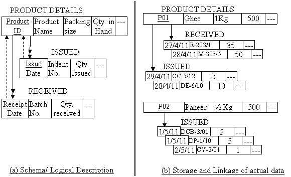
Fig. 9.11 Hierarchical Files at two levels with three record type
In the above fig 9.11(a), master record type named as PRODUCT DETAILS (root node) contains the description of milk products. There are two transaction records namely ISSUED and RECEIVED (branches) at lower level. You can see that in transaction record type ISSUED and RECEIVED, an attribute Product ID is not included since this information is drawn from the parent record type i.e. PRODUCT DETAILS. In figure 9.11(b), actual data is linked between the root node and branch node. For root Product ID P01 there are two branches of RECEIVED record type and two branches of ISSUED record type. Another root Product ID P02 has three branches of ISSUED record type.
9.5.2 Path dependency
The lower record in hierarchy (tree structure) may be incomplete in meaning without their parent. In the example discussed above (fig. 9.11 (a)), entries made in record types ISSUED and RECEIVED are incomplete without having a link to which Product ID these entries belong. Therefore, in the schema dotted lines are drawn from these record types to master record type PRODUCT DETAILS to show the path dependency.
9.6 Network Model
Hierarchical model allows one parent and one or more children relationship. Some data items and record types are more naturally modeled with more than one parent per child relationship i.e. a given data item or record type may have any number of superiors as well as any number of subordinates. Network model permits the modeling of many-to-many relationships in data. Basic data modeling construct in the network model is set construct. A set consists of an owner record type, a set name, and a member record type. A member record type can have that role in more than one set, hence the multi-parent concept is supported. An owner record type can also be a member or owner in another set. Data model is a simple network, and link and intersection record types may exist, as well as sets between them. In network structure any item or node may be linked to any other item. The network data structure looks like a tree structure, except that a dependent node called a child node may have more than one parent or owner node. So, one or more nodes may have multi-parents. Therefore a network model allows a more natural modeling of relationship between entities. There is no superior or subordinate relationship in network model as exists in hierarchical models. This kind of structure is also known as Plex structure. Fig. 9.12 given below shows some examples of network or plex structure.
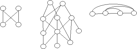
Fig. 9.12 Examples of network (plex) structure
9.6.1 Examples of M:M relationship
In real world there exist many instances including in a dairy plant where the relationship between data items or record type is many to many, for example:
· Relationship between the dairy pant and milk products, a particular plant may manufacture more than one milk product and a particular milk product may be manufactured by more than one plant for example see fig. 9.13 given below.
· Relationship between type of milk and milk products, a particular type of milk may be used in manufacturing different type of milk products and a particular milk product may be manufactured by using different type of milk.
· Relationship between machines and parts, a particular machine uses many parts and one particular part is used in many machines.
· Relationship between supplier and items, a particular supplier may supply many items and one particular item may be supplied by many suppliers.
· Relationship between course and students, a particular course may be offered by many students and a particular student may take more than one course.
The complexity of model increases with more than two entities are related with M:M relationship included in the database.
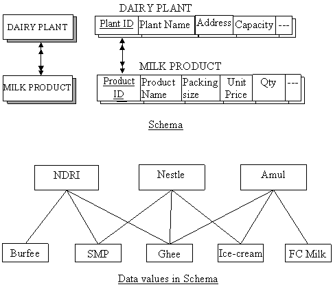
Fig. 9.13 Many to many relationships between dairy plant and milk products
9.7 Relational Model
In previous lesson two database models namely hierarchical and network were discussed. These models are structured, visualized and maintained with the help of links and pointers to show the relationship among data items or record types. These models have some advantages and disadvantages, general problem is that as the size of database grows the problem of maintaining database increases many fold. By using the links and pointers, database systems become too cumbersome, inflexible, problematic and unmanageable. The logical linkages tend to multiply as new applications are added or a user request for a new kind of query. The whole model looks like a cobweb. In 1970s, Dr. E.F. Codd, computer scientist, introduced the concept of normalization and relational model to avoid the messing of data items in hierarchical and network models. Basically, the relational models are related to user’s view of the data or logical description of data instead of physical representation of data. The physical representation and the hardware can be changed (if needed) without changing the logical/ user’s view. These concepts provided a great flexibility in designing, maintaining, updating, adding new applications and querying the database by users. Because of simplicity of management and understanding of data in relational models, relational database became very popular. Worldwide almost all databases are built up based on relational model. Relational databases are currently the predominant choice in storing data like financial records, medical records, personal information and manufacturing and logistical data.
The most natural way of recording data is in two dimensional tables. Generally at work places, data is recorded in registers and is arranged in columns and rows i.e. in tabular form. User is familiar with this style and can understand, remember and visualize data in two dimensional tables while in hierarchical or network structure relationship among data items seems to be natural but difficult to record and visualize. Therefore, practically network structure is broken down into hierarchical structure for better management of data and hierarchical structure is broken down into two dimensional tables for recording of data. A table is referred as relation in relational model. These relations form the base of relational database model.
A relation based database consists of a set of multiple tables. Each table is a relation and so a relational database can be thought of as a collection of tables. A table usually represents an object and information about that object. Objects may be physical objects or logical concepts. In each table, the rows (called tuples) represent unique entities or records and columns (called fields) represent attributes. Data values are stored at the intersection of row and column. Each named column has a domain, which is the set of values that may appear in that column. Each record in a table contains the same set of fields. Relationships are represented by common fields or attributes in different tables. Relational data structure is a mathematical model defined in terms of predicate logic and set theory. It is based on a formal theory of relational algebra. The fundamental assumption of the relational model is that all data are represented as mathematical n-ary relations; an n-ary relation being a subset of the Cartesian product of n sets. Relations have no specific order in relational database.
The relational model allows defining data structure, storage and retrieval operations and integrity constraints. Certain fields are defined as keys to index the records in a relation for fast searching and arranging the records in a particular order on key fields without creating duplicate copy of entire table. This improves the speed of searching records for specific values of that key field. Applications access data by specifying queries, which use operations such as select to identify records, project to identify attributes, and join to combine relations. Relations can be modified using the insert, delete, and update operators. New records can supply explicit values or be derived from a query. Similarly, queries identify records for updating or deleting. It is necessary for each record of a relation to be uniquely identifiable by some combination (one or more) of its attribute values. This combination is referred to as the primary key.
Relations that store data in a relational database are called "base relations". Some relations are computed by applying relational operations on base relations. Such relations are called as "derived relations". In implementations these are called "views" or "queries". Views can retrieve information from several relations and act as a single relation.
9.7.1 Example of relational database model
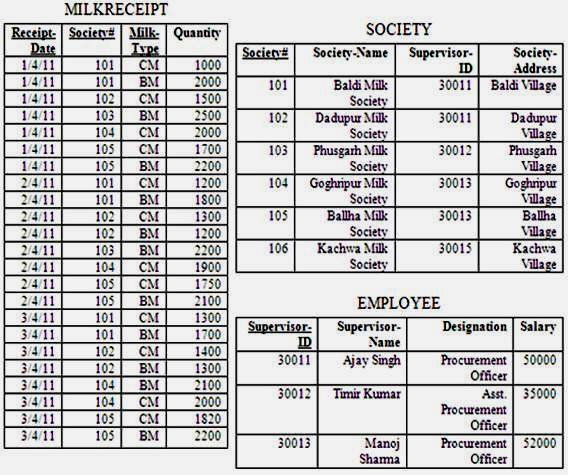
Consider a simple case of milk procurement application where milk is being collected through number of milk societies established in milk procurement area. Each society may supply CM (Cow Milk) or BM (Buffalo Milk) or both type of milk. Each society is being supervised by a staff of dairy plant. One supervisor may supervise more than one society. In this example, there are three entities or relations namely MILKRECEIPT, SOCIETY AND EMPLOYEE. Structures of these relations are described as follows:
MILKRECEIPT(Receipt-Date, Society#, Milk-Type, Quantity)
SOCIETY(Society#, Society-Name, Supervisor-ID, Society-Address)
EMPLOYEE (Supervisor-ID, Supervisor-Name, Designation, Salary)
Underlined attributes are the primary key of these relations. These relations are linked in such a way that societies supply milk to dairy and dairy plant staff supervises the societies. The relationship between MILKRECEIPT and SOCIETY is an attribute Society# and relationship between SOCIETY AND EMPLOYEE is an attribute Supervisor-ID. A sample of relational database consisting of these relations (tables) with some data values is shown in fig. 9.14 as given below:
|
|
|
|
Fig. 9.14 A view of relational database for milk procurement application |
|
9.7.2 Properties of Relational Model
A relation in relational model has following properties:
I.
Values
are atomic: This
implies that columns do not have repeating groups and cannot be broken down
further. It simplifies data manipulation.
II.
Each
row is unique: This
property ensures that each row is distinct from others. Two rows in a
relational table are not identical. Rows are uniquely identified by an
attribute or field known as primary key. Primary key may be a singly column
(field) or set of multiple columns. This property guarantees that every row in
a relational table is meaningful and that a specific row can be identified and
retrieved by specifying the value of primary key.
III.
Each
column has a unique name: Columns
represent the attributes/ characteristics of an object or entity. Each
characteristic describes some different property of an object so it should be
given a unique name to store data about these characteristics otherwise it may
create ambiguity in table. Data in a relational table is retrieved by column
names not by position of columns therefore duplicate name will create confusion
in the same table. In general, a column name need not be unique within an
entire database but only within the table to which it belongs. Moreover in
relational table the column size is also fixed.
IV.
Column
values are homogeneous: This
means that values in a column must be of the same kind. All values in column come
from the same domain. For example type of milk should have values out of CM
(cow milk) or BM (buffalo milk) if a dairy plant accept only these two type of
milk. GM (goat milk) would be a wrong data value in this column. This property
simplifies the data access because developers and users can be certain of the
type of data contained in a given column. It also ensures validation of data.
V.
The
sequence or order of columns is insignificant: This property states that the
ordering of the columns in relational table has no meaning. Columns are
retrieved by name so they can be in any order and in various sequences. This
property enables many users to share the same table without concern of how the
table is organized. It also permits the physical structure of database to
change without affecting the relational tables.
VI.
The
sequence or order of rows is insignificant: This property is analogous to the above property. To
retrieve relevant rows or records based on some condition, each row is searched
in entire table to meet the specified condition so the order of rows does not
matter. Adding new rows in a relational table (at any position, i.e., top,
bottom, in between, etc.) does not affect existing queries.
9.7.3 Relational databases terminology
I. Domain: It is used to organize and describe an attribute’s set of possible values. It is pool of values from which the actual values appearing in a column are drawn. For example values appearing in Society# column of both the MILKRECEIPT and SOCIETY tables are drawn from the underlying domain of all valid society numbers.
II. Relationship: An association between entities.
III. Degree of a relation: No. of columns in a relation.
IV. Degree of a relationship: This is number of entities associated with the relationship. The n-ary relationship is the general form for degree n. Special cases are the binary, and ternary, where the degree is 2 and 3 respectively.
9.7.4 Integrity rules
Data in a database must adhere to a set of pre-defined rules defined by an enterprise/ organization to maintain consistency in database. For example the fat% of cow milk must be in range 3% to 7%. If there is deviation then error may be either in recording the data or milk may be adulterated. The set of defined rules are called as integrity rules or constraints. In relational model there are two integrity rules as described below:
9.7.5 Entity integrity
No component of primary key value may be NULL. Primary keys perform the unique identification function in a relational database. An identifier that is wholly NULL would be a contradicting in terms, in effect, it would be saying that there was some entity that did not have any unique identification and if two entities are not identifiable from each other, then by definition these are not two, but only one entity exists.
9.7.6 Referential integrity
Let D be a domain of an attribute ‘A’ in a relation R1, then at any given time, each value of A in R1 must be either NULL or from the given domain. If A is a foreign key than it must be either NULL or any value from the set of values defined in other relation where A is primary key of that relation.
