Module 4. Database systems

Lesson 10

RELATIONAL DATABASES

10.1  Introduction

In this lesson students will learn about relational database operator for manipulating data in relational databases, and normalization techniques for designing relational databases. These topics will be useful for students to design conceptual model for development of stable database to meet the present and future requirements for an organization.

10.2  Operations on Relations

The concept of relational database is based on the theory of relational algebra therefore various types of algebraic operations can be applied on relations (tables) in relational database. Let us consider the example of relational databases discussed in previous lesson for understanding the functioning of various operations. A few commonly used operations are described as follows:

10.2.1 Insert

This operator is used to insert records in tables. Some examples of insert operation are:

• Insert-1: Insert a record for new society established in a village e.g. INSERT INTO table_name [column list] VALUES (values)

Action: Record can be easily inserted in relation SOCIETY, even if the society is not started contributing milk to dairy plant. e.g. INSERT INTO SOCIETY [column list] VALUES (values)

• Insert-2: Insert a record for receipt of milk in MILKRECEIPT relation.

Action: Record can be easily inserted in relation MILKRECEIPT, but must exist in SOCIETY relation for maintaining data integrity. For example milk received from Society#110 does not make any sense since this society number does not exist in SOCIETY relation.

10.2.2 Delete

This operator is used to remove existing records (or rows) from tables. For example:

• Delete: Suppose Society# 103 in SOCIETY relation has broken relations with dairy plant and stopped supplying of milk. So, this record can be deleted from the database by giving command e.g. DELETE FROM table_name [WHERE condition].

Action: This record can be deleted easily from SOCIETY relation the information of this society will be lost. DELETE FROM SOCIETY WHERE society# = 103.

10.2.3 Update

UPDATE allows writing queries to change data in the existing records. For example:

• Update: Change the address of the Society# 102 in SOCIETY relation.

Action: This record can be updated easily in SOCIETY relation since one change is required at one place only. UPDATE SOCIETY SET society-address = ‘new address’ WHERE society# = 102.

10.2.4 Selection

The SELECT operation retrieves records/ rows that satisfy the given conditions. A temporary view is created which can be saved in a new table or relation. This is the most commonly used operator in relational database model. It is represented by lowercase Greek letter sigma s. For example:

· Select: Execute select operation  to retrieve records/ rows of cow milk only (i.e. for milk_type equal to ‘CM’) from relation MILKRECEIPT

SELECT Receipt-Date, Society#, Milk-Type, Quantity FROM MILKRECEIPT WHERE Milk-Type = ‘CM’.

Action: Output of this Select operation is shown in fig. 10.1 given below. The output includes the records those have satisfied the condition from the original relation (fig. 9.14). Sequence of records may be original as in table

MILK
Receipt-Date	Society#	Milk-Type	Quantity
1/4/11	101	CM	1000
1/4/11	102	CM	1500
1/4/11	104	CM	2000
1/4/11	105	CM	1700
2/4/11	101	CM	1200
2/4/11	102	CM	1300
2/4/11	104	CM	1900
2/4/11	105	CM	1750
3/4/11	101	CM	1300
3/4/11	102	CM	1400
3/4/11	104	CM	2000
3/4/11	105	CM	1820

Fig. 10.1 Example of selection operation

10.2.5 Projection

This operator enables to select specified columns from a relation/ table as per requirement to create a new relation/table. The order of columns may be changed. This operator is generally represented by lowercase Greek letter pi ‘π’. In SQL it is implemented through SELECT command. For example, consider the projection  

MILK = π MILKRECEIPT(Society#, Milk-Type) of relation MILKRECEIPT.

· Projection: Create a new relation with fields Society#, Milk-Type from relation MILKRECEIPT. For this purpose execute the following SQL statement

SELECT Society#, Milk-Type FROM MILKRECEIPT

Action: Output of this projection operator is shown in fig. 10.2 given below (from original relation in fig. 9.14). The output does not have any duplicate record and the sequence of records may be as in original table.

MILK
Society#	Milk-Type
101	CM
101	BM
102	CM
103	BM
104	CM
105	CM
105	BM
102	BM
104	BM

Fig. 10.2 Example of projection operation

10.2.6 Join

The Join operation is performed to create new table (view) from two existing tables/ relations when they share a common data item. Sometimes to generate reports or queries it may be required to extract columns from two or more than two tables. These tables must be sharing common attributes. When tables are joined on a given attribute, only those records will appear in the output which shares the same value of that attribute. Therefore output may have less number of records than either of the original tables. This is called natural join. There are other types of join such as inner join, outer join etc. The Projection operator splits tables while Join operation puts together columns from different relations. Join operator is represented by ‘*’. In SQL it is implemented through SELECT command. For example, consider the Join operation on MILKRECEIPT and SOCIETY relations, MILK-SOCIETY = MILKRECEIPT * SOCIETY (Receipt-Date, Society#, Society-Name, Milk-Type, Quantity) for Milk-Type = ‘CM’.

· Join: Create a new relation with fields Receipt-Date, Society#, Society-Name, Milk-Type, Quantity from relations MILKRECEIPT and SOCIETY for cow milk only. For this purpose execute the following SQL statement

SELECT receipt-date, society#, society-name, milk-type, quantity FROM MILKRECEIPT, SOCIETY WHERE milk-type = ‘CM’

Action: Output of this Select operation is shown in fig. 10.3 given below. Output includes the records those have satisfied the condition. Sequence of records may be original as in first table.

MILK-SOCIETY
Receipt-Date	Society#	Society-Name	Milk-Type	Quantity
1/4/11	101	Baldi Milk Society	CM	1000
1/4/11	102	Dadupur Milk Society	CM	1500
1/4/11	104	Goghripur Milk Society	CM	2000
1/4/11	105	Ballha Milk Society	CM	1700
2/4/11	101	Baldi Milk Society	CM	1200
2/4/11	102	Dadupur Milk Society	CM	1300
2/4/11	104	Goghripur Milk Society	CM	1900
2/4/11	105	Ballha Milk Society	CM	1750
3/4/11	101	Baldi Milk Society	CM	1300
3/4/11	102	Dadupur Milk Society	CM	1400
3/4/11	104	Goghripur Milk Society	CM	2000
3/4/11	105	Ballha Milk Society	CM	1820

Fig. 10.3 Example of Join operation on MILKRECEIPT and SOCIETY

Similarly the result of join operation on SOCIETY and EMPLOYEE relation is shown in fig. 10.4 given below:

SOC-EMP = SOCIETY* EMPLOYEE (Society#, Supervisor-ID, Supervisor-Name, Salary)

SELECT society#, supervisor-ID, supervisor-Name, salary FROM SOCIETY,  EMPLOYEE

SOC-EMP
Society#	Supervisor-ID	Supervisor-Name	Salary
101	30011	Ajay Singh	50000
103	30012	Timir Kumar	35000
104	30013	Manoj Sharma	52000

Fig. 10.4 Example of Join operation on MILKRECEIPT and SOCIETY

10.2.7  Union

This operator combines the records of two relations and removes all duplicate records from the result.

10.2.8  Intersection

This operator produces a set of common records from two relations.

10.2.9  Cartesian product

Cartesian product of two relations is a join that is not restricted by any criteria, resulting in every record of the first relation being matched with every record of the second relation.

Many updates and queries are accomplished by combining multiple tables in various ways, thus providing an extremely powerful access capability. For example, MILKRECEIPT and SOCIETY relations can be joined along with select and project operations. It is evident from the foregoing discussion that relational approach is conceptually straight forward in design as compared to the other two approaches. In addition, the underlying theory is elegant and precise allowing for complex natural relations to be represented clearly.

In a hierarchical or network model the connections and relationships are in the data structure. If a new relationship is to be added, new connections and access paths must be established. In a relational database, access paths need not be pre-determined. Creating new relations simply requires a joining of tables. Relational databases are therefore the most flexible and useful for unplanned and ad-hoc queries. The pre-determined relationships of the hierarchical or the network structures require more complex data definition language (DDL) and data manipulation language (DML). Maintenance is more difficult. The relational model data definition and data manipulation languages are simple and user oriented. Maintenance and physical storage are fairly simple.

10.3  Conversion of Hierarchical Model (Tree Structure) into Relational Model

A hierarchical model (tree structure) can be easily converted into relational model with minimal redundancy. For example, consider a tree structure as given in fig. 9.11, PRODUCT DETAIL record type is having 1:M relationship with ISSUED and RECEIVED record type. Each record in ISSUED and RECEIVED relation is identified by a link from an attribute Product ID in PRODUCT DETAIL i.e. for every record in ISSUED and RECEIVED there is path dependency from PRODUCT DETAIL. To convert this trees structure into relational model, path dependency is to be removed by introducing one more attribute Product ID  in relations ISSUED and RECEIVED. There will tree relations in the relational database model as shown in fig. 10.5.

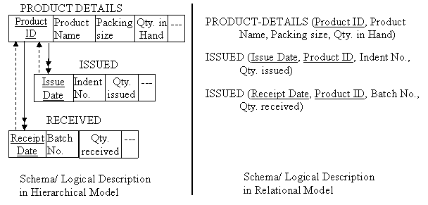
Fig. 10.5 Conversion of hierarchical model into relational model

10.4 Conversion of Network Model (Plex Structure) into Relational Model

A network model (plex structure) can be converted as easily as hierarchical model into relational model. Consider an example of network model shown fig. 9.13 and as discussed in previous lesson, there are two record types namely DAIRY PLANT and MILK PRODUCT. These records are linked to each other with M:M relationship and association between them is Unit Price of milk product fixed by different diary plants. This attribute is recognized by two items e.g. Product ID and Plant ID. To convert this structure into relational model, a new record type is created to store the association of existing two record types as shown in fig. 10.6.

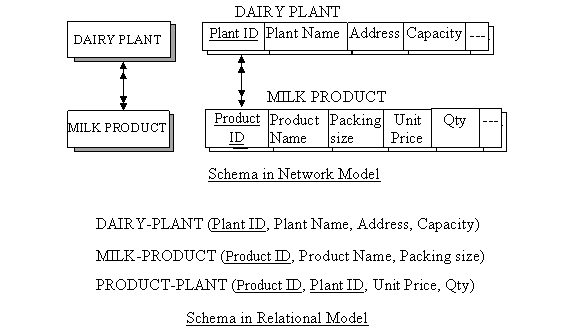
Fig. 10.6 Conversion of network model into relational model

10.5 Advantages of Relational Database Model

• Easy to use and understand: It very easy to use and understand than other models. It is easy to add information in the form of table.
• Data independence: In comparison with Hierarchical or Network model, it is easy to achieve data independence in relational model.
• Flexible: Relational model is flexible to add new data items or new tables/ relations etc.
• Security: Data security measures can be implemented easily.
• Ad-hoc query: Ad-hoc unforeseen queries can be generated and process easily.

10.6 Disadvantages of Relational Database Model

• Complex: It is complex to design and develop and then creating and maintaining relationships among relations.
• Requires more memory: Extra memory is required to create and store indexes for searching and retrieving data. 
• Hardware cost: Powerful hardware is required to process data.
• Time consuming: Extra time is required to search a record because records are searched sequentially.

10.7 Normalization

Normalization is a design technique that is widely used as a guide in designing relational databases. Normalization is a natural process of grouping related data and then placing in different tables to minimize duplication of data. Normalization process has been defined by different researchers in their own way. Some important descriptions are as follows:

• Normalization is a process by which attributes are grouped together to form a well structured relation.
• Normalization is a process of simplifying the relationship between the data elements in a record.
• Normalization is basically a process of efficiently organizing data in a database with the objectives to eliminate redundant data (for example storing the same data in more than one table) and to ensure data dependencies make sense (only storing related data in a table). These objectives are important as they reduce the amount of space of database and ensure that data is logically stored.
• Normalization is a step by step process for replacing association (1: M and M: M) between data items in two dimensional tabular forms (or flat-file representation) by storing data in separate files to minimize redundancy and simplify basic database file management.
• The purpose of normalization is to produce a stable set of relations that is a faithful model of the operations of an enterprise. By following the principle of normalization we can achieve a design that is highly flexible, allowing the model to be extended.
• The practice of storing data in separate two dimensional tables or flat files to minimize redundancy and simplify basic database file management is called normalization
• Normalization is a process of breaking a relation into sub relations such that the sub relations so formed are free from insert, delete, and update anomalies.

From above descriptions, finally we can say that normalization is:

“Normalization is a step by step process for replacing association (1:M and M:M) between data items in two dimensional tabular forms (i.e. flat-file representation) by storing data in separate files to minimize redundancy and simplify basic database file management. The overall aim is to produce a stable set of relations that is a faithful model of the operations of an enterprise. Normalization process involves the removing:

· Redundant data

· Partial dependencies

· Transitive dependencies

By following the principles of normalization, one can achieve a database design that is highly flexible; reliable; extendable; free from insert, delete, and update anomalies; and easy to implement”.

Normalization theory is based on the concepts of normal forms. A relational table is said to be in a particular normal form if it satisfies a certain set of constraints. There are currently five normal forms termed as 1^st, 2^nd, 3^rd, Boyce-Codd Normal Form (BCNF),  4^th and 5^th normal form (NF) respectively. In practice, majority of the relations become free from different kind data anomalies when they are in 3^rd NF and generally, it has been observed by practitioners that entities that are in 3^rd NF are also in 4^th and 5^th NF. So, first three forms are sufficient to design a good and stable database for an organization. Therefore for simplicity, we will discuss only first three normal forms in this lesson. Normalization process has following goals:

I. The goal of normalization is to create a set of relational tables that are consistent and free of redundant data.

II. The normalization rules are designed to prevent update anomalies and data inconsistencies.

III. The normalized design enhances the data integrity by minimizing the redundancy and inconsistency but at cost of performance for certain retrieval application. 

10.8  Important Terms Used in Normalization Process

Before understanding the normal forms, it is important to understand few key terms which forms the base of normalization concept:

10.8.1 Functional dependencies

The concept of functional dependencies is the basis for the first three normal forms. Functional dependency describes a relationship between attributes in a single relation. An attribute is functionally dependant on another if we can use the value of one attribute to determine the value of another. So functional dependency may be defined as: “An attribute B of a relation R is functionally dependent on attribute A or R if, at every instant of time, each value in A has no more than one value in B associated with it in relation R”.  Or in other words it can be defined as

“A column, Y of a relational table R is said to be functionally dependent on column X of R, if and only if each value of X in R is associated with precisely one value of Y at any given time. X and Y may be composite”. Saying that column Y is functionally dependent on X is the same as saying the values of column X identify the values of column Y. If column X is a primary key, then all columns in relational table R must be functionally dependent on X.

Symbol → is used to indicate a functional dependency. → is read as functionally determines. One can read X → Y as, "X determines Y". Functionality is shown graphically in fig. 10.7 given below:

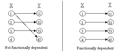
Fig. 10.7 Graphical representation of functional dependencies

Example-1: Consider a relation of containing employee details working in different projects running in a dairy plant.

EMPLOYEE (Employee-ID, Employee-Name, Qualification, Phone-Number, Salary, Project-ID, Completion-Date)

The functional dependencies in this relation are as follows in fig. 10.8:

Attributes	Functional Dependency	Attribute name	Symbolic Trems
*Employee -ID	Dependent on	Employee-Name	Employee-ID → Employee-Name
*Employee-Name	Dependent on	Employee-ID	Employee-Name → Employee-ID
Qualification	Dependent on	Employee-ID	Employee-ID → Qualification
Phone-Number	Dependent on	Employee-ID	Employee-ID → Phone-Number
Salary	Dependent on	Employee-ID or Employee- Name	Employee-ID → Salary (but reverse is not true)
Project-ID	Dependent on	Employee-ID or Employee- Name	Employee-ID → Employee-Name → Project-ID (but reverse is not true)
Completion-Date	Dependent on	Employee-ID or Employee-Name or Project-ID	Employee-ID → Completion-Date Employee-Name → Completion-Date Project-ID → Completion-Date (but reverse is not true)

Fig. 10.8 Description of functional dependencies for relation EMPLOYEE

Employee-Name is functionally dependant on Employee-ID because Employee-ID can be used to determine the value of Employee-Name and one Employee-ID will be related to only one name (Employee-ID → Employee-Name). Employee-ID is not functionally dependent on Salary because more than one employee could have the same salary. Similarly, Employee-ID is not functionally dependent on Project-ID or Completion-Date. Completion-Date is functionally dependent on Project-ID only. No other attributes in this relation is fully dependent on project-ID except Completion-Date. The asterisks indicate prime attributes (member for candidate key)

Example-2: An attribute can be functionally dependent on group of attributes rather on a single attribute. Consider a relation of employees where a particular employee is working in more than one section of a dairy plant.

EMP-SECTION (Emp-ID, Section-ID, Emp-Name, Section-Name, Total-Work-Hrs) 

The functional dependencies in this relation are as follows in fig. 10.9:

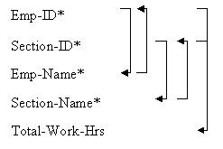
Fig. 10.9 Description of functional dependencies for relation EMP-SECTION

Here Total-Work-Hrs is functionally dependant on Emp-ID and Section-ID. Either Emp-ID or Section-ID individually is not competent to identify the value of Total-Work-Hrs. The asterisks indicate prime attributes (member for candidate key)

Example-3: Consider a relation having details of milk product in a dairy plant

PRODUCT (Product-ID, Product-Name, Packing-Size, Unit-Price, FAT%, SNF%)

The functional dependencies in this relation are as follows in fig. 10.10:

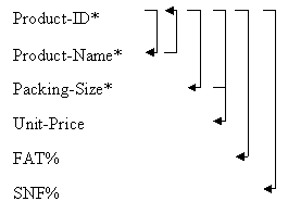
Fig. 10.10 Description of functional dependencies for relation PRODUCT

Product-Name is functionally dependant on Product -ID because Product -ID can be used to determine the value of Product -Name and one Product ID will be related to only one product (Product-ID → Product-Name). Unit price is dependent on Product-ID as well as packing size. The asterisks indicate prime attributes (member for candidate key)

Example-4: Consider a relation having details of supply source of various machine parts used in a dairy plant. These parts are supplied by different suppliers.

SUPPLY-SOURCE (Supplier-ID, Part-ID, Supplier-Name, Supplier-Address, Price) 

The functional dependencies in this relation are as follows in fig. 10.11:

Fig. 10.11 Description of functional dependencies for relation PRODUCT

Here Price is functionally dependant on Supplier-ID and Part -ID because different suppliers may supply the same part at different price. So both Supplier-ID and Part -ID attributes are used to identify the attribute Price. The asterisks indicate prime attributes (member for candidate key)

10.8.2 Full functional dependency

This applies to tables with composite keys and can be defined as “An attributes or a collection of attributes B of a relation R can be said to be fully functionally dependent on another collection of attributes A; of relation R if B is functionally dependent on the whole of A but not on any subset of A”.  Or in other words as

“Column Y in relational table R is fully functional dependent on X of R if it is functionally dependent on whole X and not functionally dependent on any subset of X. Full functional dependency means that when a primary key is composite, made of two or more columns, then the other columns must be identified by the entire key and not just some of the columns that make up the key”.

For example, consider the relation EMP-SECTION given in example-2 above (fig. 10.9), an attribute Total-Work-Hrs is fully functional dependent of the combination of key (Emp-ID + Section-ID) because to know that how many hours a particular worker has worked in a particular section, information from both of these key fields is required. Neither Emp-ID, alone nor Section-ID alone can identify the attribute Total-Work-Hrs. Other fields such as Emp-Name, is fully functional dependent on Emp-ID alone and Section-Name is fully functional dependent on Section-ID alone. Similarly you see in example-3 and example-4 discussed above.

10.8.3 Partial dependencies

Partial dependencies might occur in a relation that contains a composite primary key and some attributes are dependent on part of the primary key rather than entire key. In that situation, any data item that is not dependent on all key fields should be removed into a separate database file. For example consider the relation SUPPLY-SOURCE as discussed in example-4 above (fig. 10.11). The primary key of this relation is combination of Supplier-ID + Part-ID attributes. As seen in fig. 10.11, attributes Supplier-Name and Supplier-Address are functionally dependent on part of the key attribute i.e. Supplier-ID not on the whole key. Only an attribute Price of the relation is totally dependent on the whole key i.e. Supplier-ID + Part-ID. Therefore, attributes Supplier-Name and Supplier-Address must be removed from relation SUPPLY-SOURCE and stored in some other relation with key attribute Supplier-ID only.   

10.8.4 Partial key

It is a set of attribute that can be uniquely identifying weak entities and that are related to same owner entity. It is sometime called as Discriminator.

10.8.5 Artificial key

If no obvious key either stands alone or composite is available, then the last resort is to simply create a key, by assigning a unique number to read each record or occurrence. Then it is known as developing an artificial key.

10.9 First Normal Form (1NF)

The normalization process starts with natural instinct of arranging data items into two dimensional tables by breaking up of data items into smallest possible units. Repeating data items are removed from the table and are placed in a new separate table. A key field is used to link these two partitioned tables. After that a database is said to be in first normal form (1NF). More precisely, “A relation R is said to be in first normal form (1NF) if and only if all underlying domains contain atomic values only”.  Thus 1NF describes the tabular format in which:

· All occurrences of a record type must contain the same number of fields.

· All attributes are atomic.

· All the key attributes are defined.

· There are no repeating groups in the table.

· All attributes are dependent on primary key.

For example consider the relation EMPLOYEE as discussed above in example-1 (figure-26.1). At first glance this relation seems to be in 1NF, if we assume that the attributes Employee-Name, Phone-Number and Qualification are atomic i.e. these cannot be braked down further. Similarly if we assume that one employee may have only value for attributes Phone-Number and Qualification respectively. In real word such assumptions are not realistic. Practically, employee name may be considered as a combination of three fields namely First-Name, Second-Name, and Last-Name.; employee phone number may consist of Country-Code, STD-Code, and Actual-Number; and qualification may be broken into Exam-Passed, Year, and Marks-Obtained.   Moreover one employee can have more than one qualification and phone number. Therefore as per the above definition of 1NF this relation can be redesigned as follows:

EMPLOYEE (Employee-ID, First-Name, Middle-Name, Last-Name, Salary, Project-ID, Completion-Date)

QUALIFICATION (Employee-ID, Sr-No, Exam-Passed, Year, Marks-Obtained)

PHONES (Employee-ID, Sr-No, Country-Code, STD-Code, and Actual-Number)

In the relations QUALIFICATION and PHONES, a new dummy field namely Sr-No is added and concatenated with key field Employee-ID to identify a record uniquely in these tables.

10.10 Second Normal Form (2NF)

The definition of second normal form states that only the data items those are directly relevant to the entire key fields (in case of composite key) should be in relational table and other data items must be split into separate tables. This means that in 2NF each field in a table with composite primary key must be directly related to the entire key not on a part of primary key. More precisely, “A relation R is in 2NF if it is in 1NF and every non-prime attributes of R is fully functionally dependent on primary key of R”.

For example consider the relation EMPLOYEE as discussed above in 1NF. The partitioned tables are already in 2NF since the primary key Employee-ID of relation EMPLOYEE consists of only one attributes, and every non-prime attributes are fully dependent on the primary key. In other relations QUALIFICATION and PHONES all non prime attributes are fully dependent on the composite primary key, i.e., Employee-ID + Sr-No respectively.

The relation EMP-SECTION in fig. 10.9, it is already in 2NF since the attribute Total-Work-Hrs is fully functionally dependant on whole primary key i.e. on the combination of Emp-ID + Section-ID. Similarly it is dependent on combination of candidate keys like Emp-Name, Section-Name.

The following relation described in example-4 (fig. 10.11) is not in 2NF:

SUPPLY-SOURCE (Supplier-ID, Part-ID, Supplier-Name, Supplier-Address, Price)

The relation has a composite primary key Supplier-ID + Part-ID. Attributes Supplier-Name and Supplier-Address are functionally dependent only on part of the key i.e. Supplier-ID not on whole primary key. The attribute Price is fully functional dependent on combined key. When a relation is not in 2NF then there will be few problems related to data updates in such relations as discussed below:

· Details of a supplier cannot be entered in database until that supplier supplies some parts.

· Suppose a supplier is supplying only a single part and due to some reasons he temporarily stops the supply of that part, then deletion of records for that part will also remove the information of supplier. But it would be desirable to preserve the details of supplier in an organization for future use.

· Suppose a supplier changes his address then all records in the database are to be updated for that supplier. This would be required to be done at many places (redundancy), time consuming and may lead to inconsistency in the database.

These anomalies can be solved by splitting the relation into two relations as follows:

SUPPLY-SOURCE (Supplier-ID, Supplier-Name, Supplier-Address)

SUPPLY-SOURCE (Supplier-ID, Part-ID, Price)

In these relations all non prime attributes are fully functionally dependent on primary key of the relations. Similarly the relation as given below and discussed in example-3 (fig. 10.10) is not in 2NF

PRODUCT (Product-ID, Product-Name, Packing-Size, Unit-Price, FAT%, SNF%)

This relation can be brought into 2NF by splitting into two relations as follows:

PRODUCT (Product-ID, Product-Name, FAT%, SNF %)

PRODUCT-PACKING (Product-ID, Packing-Size, Unit-Price)

10.11  Third Normal Form (3NF)

The problems related to data updates as discussed in above section can occasionally occur even if a relation is in second normal form. To remove such anomalies database relation is further refined by using the third normalization step. The third normal form requires that all columns in a relational table should be dependent only on the primary key. A more formal definition is: “A relation R is in third normal form (3NF) if it is already in 2NF and every non-key attributes of R is non-transitively dependent on each candidate key of R”. When all the transitive dependencies have been removed from the relation; the database is said to be in the third normal form.

10.11.1  Transitive dependency

A transitive dependency occurs when non-key attribute that is a determinant of primary key is also the determinant of other attribute. This means that transitive dependency in a relation occurs due to those attributes that are occasionally (though not always) dependent on some other non key field in the same relation.

In symbolic term it can be defined as “suppose that A, B and C are three attributes or distinct collections of attributes of a relation R, If C is functionally dependent on B and B is functionally dependent on A, then C is functionally dependent on A. If the inverse mapping is non-simple (i.e., if A is not functionally dependent on B or B is not functionally dependent on C), then C is said to be transitively dependent on A. The transitive dependency may be removed by splitting the relation into two parts as shown in fig. 10.12 given below:

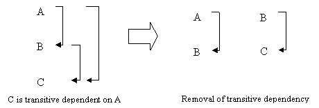
Fig. 10.12 Representation of transitive dependency and its removal

For example consider the relation EMPLOYEE as discussed above in example-1 (fig. 10.8). This relation was further converted into three relations after passing through the first normalization form as given below:

· EMPLOYEE (Employee-ID, First-Name, Middle-Name, Last-Name, Salary, Project-ID, Completion-Date)

· QUALIFICATION (Employee-ID, Sr-No, Exam-Passed, Year, Marks-Obtained)

· PHONES (Employee-ID, Sr-No, Country-Code, STD-Code, and Actual-Number)

Automatically this relation is also in 2NF as it fulfills the requirement of second normalization form. But there is a problem when the conditions of 3NF are applied on these relations especially in relation EMPLOYEE. In this relation, attribute Project-ID is functionally dependent on Employee-ID and attribute Completion-Date is functionally dependent on Project-ID which is a non key attribute. Further on analyzing the reverse relationship it is observed that is Employee-ID in not functional dependent on Project-ID similarly Project-ID is not functional dependent on Completion-Date. It means the inverse mapping is non-simple. Therefore, Completion-Date is transitively dependent on Employee-ID. To remove the transitive dependency the relation EMPLOYEE may be split into two relations as follows:

· EMPLOYEE (Employee-ID, First-Name, Middle-Name, Last-Name, Salary, Project-ID)

· PROJECT (Project-ID, Completion-Date)

Thus after going through 3 phases of normalization process i.e. 1NF, 2NF and 3NF the original relation would be converted into four relations as given below:

· EMPLOYEE (Employee-ID, First-Name, Middle-Name, Last-Name, Salary, Project-ID)

· QUALIFICATION (Employee-ID, Sr-No, Exam-Passed, Year, Marks-Obtained)

· PHONES (Employee-ID, Sr-No, Country-Code, STD-Code, and Actual-Number)

· PROJECT (Project-ID, Completion-Date)

When a relation is not in 3NF then there will be few problems related to data updates in such relations as discussed below:

· Unless an employee is hired in a project, the project detail can be entered in database. This means that for a new project if employee is not recruited, the details of the project like completion date cannot be entered because this information is a part of the employee relation.

· If all employees working in a project left the job then their records will also be deleted from the database. The deletion of records may lead to the loss of an important information about the project i.e. completion date because this information is a part of the employee relation.

· Suppose a particular project is extended by another one year more, then this change has to be incorporated in all relevant records. This may lead to inconsistency in the database.

After removing transitive dependency the original relation is converted into two new relations.  In each relation the attributes are fully functional dependent on the prime attribute of the relation. These converted relations will not have the data anomalies as discussed above. Thus, the database emerging out after passing through the three steps of normalization will be flexible; reliable; extendable; free from insert, delete, and update anomalies; and easy to implement.