Module 1.
Descriptive statistics
Lesson 3
MEASURES OF CENTRAL TENDENCY
3.1 Introduction
The collected data as such are not suitable to draw conclusions about the mass from where it has been taken. Some inferences about the population can be drawn from the frequency distribution of the observed values. One of the important objectives of statistical analysis is to determine various numerical measures which describe the inherent characteristics of a frequency distribution. The averages are the measures which condense a huge unwieldy set of numerical data into single numerical value, are representative of the entire distribution. Hence, in finding a central value, the data are condensed into a single value around which most of the values tend to cluster. Commonly, such a value lies in the centre of the distribution and is termed as central tendency.
3.2 Measure of Central Tendency or Average
One of the most important objectives of the statistical analysis is to get one single value that describes the characteristic of the entire mass of unwieldy data. Such a value is called the ‘Central Value’ or ‘an average’. The word ‘Average’ is very commonly used in everyday conversation. For example we talk of average milk yield of a cow, average fat content of milk , average height or life of an Indian, average income etc. When we say ‘he is an average student’ what it means is that he is neither very good nor very bad, just a mediocre type of student. Similarly, when we talk of average size of butter or cheese packet being sold through a retail outlet what we mean is that the size of packet which is being sold to maximum number of individuals by the retail outlet that means it is the modal size. However, in statistics the term average has a different meaning. According to Croxton and Cowden “An average value is a single value within the range of the data and is used to represent all of the values in the series. Since an average is within the range of the data, it is sometimes called a measure of central value.” It may be defined as that value of a distribution which is considered as the most representative of the series or typical value for a group. Such a value is of great significance because
· It depicts the characteristic of the whole group
· It facilitates comparison
Averages are sometime referred to as a measure of location since they enable us to locate the position or place of the distribution in question.
Requisites of a good average
· It should be rigidly defined.
· It should be easy to understand and calculate.
· It should be based on all the observations.
· It should not be unduly affected by extreme observations.
· It should be suitable for further mathematical treatment.
· It should be least affected by fluctuations of sampling.
The various measures of central tendency or averages are discussed below:
3.3 Arithmetic Mean
Its value is obtained by adding together all the items and dividing it by the total number of observations. If X1, X2, . . . . . , Xn are n values of a variable X, then the arithmetic mean (A.M.) in case of raw data, is defined as
![]()
In case of frequency distribution
|
Xi |
X1 |
X2 |
X3 |
--- |
Xn |
|
fi |
f1 |
f2 |
f3 |
--- |
fn |
If the value X1 occurs f1 times, the value X2 occurs f2 times, …, the value Xn occurs fn times, then the arithmetic mean is given by

where, ![]()
3.3.1 Arithmetic mean in case of grouped data
In case of grouped data, arithmetic mean can be calculated by applying any of the following methods:
i) Direct Method ii) Short cut Method iii) Step-deviation Method
3.3.1.1 Direct method
· Multiply each value of Xi (the mid value of the class) by the corresponding frequency fi.
· Obtain
the sum of the products ![]() .
.
· Divide this sum of products by the total frequency (N) so as to get mean.
Example 1: Find the mean from frequency distribution given in example 2 of Lesson 2.
Solution: Prepare the following table and calculate arithmetic mean as follows:
|
Class Interval |
Mid-value
(Xi) |
frequency
(fi) |
fi Xi |
|
1630-1730 |
1680 |
17 |
28560 |
|
1730-1830 |
1780 |
19 |
33820 |
|
1830-1930 |
1880 |
23 |
43240 |
|
1930-2030 |
1980 |
16 |
31680 |
|
2030-2130 |
2080 |
14 |
29120 |
|
2130-2230 |
2180 |
7 |
15260 |
|
2230-2330 |
2280 |
2 |
4560 |
|
2330-2430 |
2380 |
2 |
4760 |
|
Total |
|
100 |
191000 |
![]()
3.3.1.2 Short–cut method (Change of Origin)
If the values of X or/and f are large, the calculation of mean by direct method is quite tedious and time consuming. In such a case the calculations can be reduced to a great extent by using short cut method. This method consists in taking deviations of the given observations from any arbitrary value A. The formula for calculation of the arithmetic mean is
![]()
Where A is arbitrary mean, di’
= Xi – A i.e.
deviation from the arbitrary or assumed mean.
3.3.1.3 Step-deviation method (Change of origin and scale)
In case of grouped frequency
distribution, with class intervals of equal magnitude, the calculations are
further simplified by taking;![]() where Xi is the mid value of the
class and h is the common magnitude or width of the class intervals. So the
formula for calculating mean is
where Xi is the mid value of the
class and h is the common magnitude or width of the class intervals. So the
formula for calculating mean is![]() .
The procedure is illustrated in the example 2. It will be seen that the answer
in each of the three cases is the same. The step-deviation method is the most convenient
method on account of simplified calculations.
.
The procedure is illustrated in the example 2. It will be seen that the answer
in each of the three cases is the same. The step-deviation method is the most convenient
method on account of simplified calculations.
Example 2: Solve example 1 with short-cut and step-deviation method.
Solution: Prepare the following table and calculate arithmetic mean as follows:
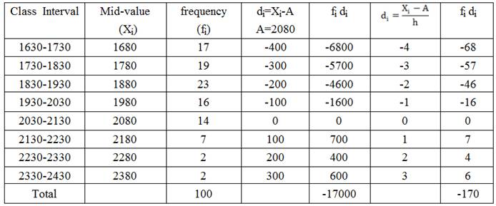
a) Short-cut
method: A=2080
![]()
b)
Step-Deviation Method: A=2080, h=100
![]()
3.3.2 Mathematical properties of arithmetic mean
i)
The
algebraic sum of the deviations of the given set of observations from their
arithmetic mean is zero i.e. ![]() .
.
ii) If
n1 and n2 are the sizes and ![]() are
the respective means of two series then the pooled mean
are
the respective means of two series then the pooled mean ![]() of the combined series of size (n1+n2)
observations is given by:
of the combined series of size (n1+n2)
observations is given by:
![]()
iii) The sum of the squares of deviations of the given set of observations, when taken from their arithmetic mean, is minimum.
3.3.3 Merits of arithmetic mean
· The A.M. is rigidly defined
· It is based on all the observations
· It is easily calculated from the given data
· It is least affected by fluctuations of sampling
· It is suitable for further mathematical treatment. The average of two or more series can be obtained from the averages of the individual series.
3.3.4 Demerits of arithmetic mean
· The strongest drawback of arithmetic mean is that it is very much affected by extreme observations.
· In a distribution with open end classes the value of mean cannot be computed without making assumptions regarding the size of class.
· It can neither be located by inspection nor graphically.
· It cannot be used for qualitative type of data such as intelligence, honesty, flavor, overall acceptability of dairy product etc.
· Arithmetic mean cannot be obtained if a single observation is missing or lost.
· In a skewed distribution, usually arithmetic mean is not representative of the distribution.
3.4 Geometric Mean
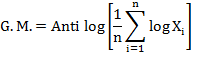
The geometric mean (usually denoted by G.M.) of a set of n observations is the nth root of their product. If X1, X2, . . . , Xn are n values of a variable X, none of them being zero, then the geometric mean, G.M. is defined by
![]()
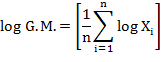
Thus logarithm of G.M. of a set of observations is the arithmetic mean of their logarithms.
If
X1, X2, . . . , Xn occurs f1,
f2 . . . , fn times respectively then
![]()
![]()
3.4.1 Merits of geometric mean
· It is rigidly defined
· The G.M. is based on all observations of a series.
· It is not much affected by fluctuations of sampling.
· It is suitable for further mathematical treatment.
· Unlike arithmetic mean which has a bias for higher values, geometric mean has bias for smaller observations.
· As compared with Arithmetic mean, Geometric mean is affected to a lesser extent by extreme observations.
3.4.2 Demerits of geometric mean
· Computations are difficult
· It is not simple to understand
· It does not give equal weight to every item.
· It cannot be calculated if the number of negative values is odd as well as some value is zero.
3.4.3 Use of geometric mean
It is most appropriate average when dealing with ratios, percentages and rate of increase between two periods. It is applied when increase or decrease in time is proportional e.g. growth of population is proportional to the time, increase in bacterial population is proportional to the time and rate of interest. Geometric Mean is used in the construction of Index numbers.
3.5 Harmonic Mean
If X1, X2,
. . . , Xn are n values of a variable X, then their Harmonic Mean,
abbreviated as H.M. is defined by
![]()
In other words Harmonic
Mean is the reciprocal of the arithmetic mean of the reciprocals of the given
observations. In case of grouped frequency distribution, harmonic mean is given
by
![]()
3.5.1 Merits of harmonic mean
· It is rigidly defined
· The H.M. is based on all observations of a series.
· It is not much affected by fluctuations of sampling.
· It is suitable for further mathematical treatment.
· Since the reciprocals of the values of the variable are involved, it gives greater weight age to smaller observations and as such is not very much affected by one or two big observations.
3.5.2 Demerits of harmonic mean
· Computations are difficult and not simple to understand.
· It cannot be calculated if any one of the observations is zero.
· It is not a representative figure of the distribution unless the phenomenon requires greater weight age to be given to smaller values.
3.5.3 Use of harmonic mean
H.M. is used in finding averages involving speed, time, price and ratios. It is useful for computing the average rate of increase of profits of a concern or average speed at which a journey has been performed or the average price at which an article has been sold. The rate usually indicates the relation between two different types of measuring units that can be expressed reciprocally. The H.M. is used for the problems about work, time and rate, where the amount of work is held constant and the average rate is required, or in problems about total cost, number of persons and per capita cost is called for or in problems of similar nature involving rates.
The arithmetic mean
(A.M.), the geometric mean (G.M.) and the harmonic mean (H.M.) of a series of n
observations are connected by the relation A.M. ≥ G.M. ≥ H.M.
The computation of G.M. and H.M. is illustrated in example 3.
Example 3: Find G.M. and H.M. of data given in example 1.
Solution: Prepare the following table and calculate G.M. and H.M. as follows:
|
Class Interval |
Mid-value (Xi) |
frequency (fi) |
log Xi |
fi log Xi |
|
|
|
1630-1730 |
1680 |
17 |
3.2253 |
54.8303 |
0.0006 |
0.0101 |
|
1730-1830 |
1780 |
19 |
3.2504 |
61.7580 |
0.0006 |
0.0107 |
|
1830-1930 |
1880 |
23 |
3.2742 |
75.3056 |
0.0005 |
0.0122 |
|
1930-2030 |
1980 |
16 |
3.2967 |
52.7466 |
0.0005 |
0.0081 |
|
2030-2130 |
2080 |
14 |
3.3181 |
46.4529 |
0.0005 |
0.0067 |
|
2130-2230 |
2180 |
7 |
3.3385 |
23.3692 |
0.0005 |
0.0032 |
|
2230-2330 |
2280 |
2 |
3.3579 |
6.71587 |
0.0004 |
0.0009 |
|
2330-2430 |
2380 |
2 |
3.3766 |
6.75315 |
0.0004 |
0.0008 |
|
Total |
|
100 |
|
327.9316 |
|
0.0528 |
![]()
![]()
![]()
From example 2 and example 3 one
can verify that A.M. ≥ G.M. ≥ H.M.
3.6 Median (Positional Average)
The median is defined the measure of the central value when arranged in ascending or descending order of magnitude. According to L.R. Connor “The median is that value of the variate which divides the group in two equal parts, one part comprising all the values greater and the other, all values less than median”. Thus, as against arithmetic mean which is based on all the items of the distribution, the median is only positional average i.e. its value depends on the position occupied by a value in the frequency distribution.
3.6.1 Calculation of median
3.6.1.1 Ungrouped data
When
the total numbers of observations are odd, then the median is the middle value
after the observations are arranged in ascending or descending order of
magnitude. If the number of observations is equal to n, then the value of
((n+1)/2)th item gives the value of median e.g. the median of 5
observations 65,69,52,58,45 i.e. 45,52,58,65,69 is 58. When the total number of
observations is even then median is obtained as the arithmetic mean of the two
middle observations after they are arranged in ascending or descending order of
magnitude. If number of observations are say 2n, then the arithmetic average of
nth and (n+1)st (central items) gives the value of
median. If it is n then median is the arithmetic average of ![]() and
and
![]() values e.g. the median of 6 observations
65,69,52,58,45,67 i.e. 45,52,58,65,67,69 is arithmetic mean of 58 and 65 which
is equal to 61.5.
values e.g. the median of 6 observations
65,69,52,58,45,67 i.e. 45,52,58,65,67,69 is arithmetic mean of 58 and 65 which
is equal to 61.5.
3.6.1.2 Grouped data
Steps involved for its computation are:
1) Prepare less than cumulative frequency(c.f. ) distribution table
2) Find N/2.
3) Find cumulative frequency just greater than N/2
4) The class corresponding to step 3 contains the median value and is called the median class.
The median for a grouped series is given by the following formula:
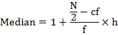
Where: l is the lower limit of the median class
f is the frequency of the median class
h is width of the class interval
c.f. is the cumulative frequency of the class preceding the median class.

The computational procedure is illustrated in Example 3.4.
3.6.2 Merits of median
· It is rigidly defined.
· It is easily understood, very readily calculated and can exactly be located.
· It is readily obtained without the necessity of measuring all the objects.
· It is not affected by abnormally large or small values of the variable.
· Median can be computed while dealing with a distribution with open end classes.
· It can be determined by mere inspections and can be computed graphically.
· The median gives the best results in a study of direct qualitative measurements such as intelligence, honesty etc.
3.6.3 Demerits of median
· The median does not lend itself to algebraic treatment. The median of several series by combining the medians of the component series cannot be computed.
· Median being positional average is not based on each and every item of the observations.
· Median is relatively less stable than mean, particularly for small samples since it is affected more by fluctuations of sampling as compared to arithmetic mean.
3.7 Quartiles
Quartiles
are those values of the variate which divide the total frequency into four equal
parts. Obviously there will be three such points Q1, Q2 and
Q3 such that Q1≤ Q2 ≤ Q3 termed
as the three quartiles. Q1is known as the lower or first
quartile and is the value which has 25% of the items of the distribution below
it and consequently 75 percent of the items are greater than it. Q3
is known as the upper or third quartile and has 75percent of the
observations below it and consequently 25 percent of the observations above it.
![]()
3.8 Deciles
Deciles
are those values of the variate which divide the total frequency into 10 equal
parts. The formula for obtaining jth Decile (Dj) in case
of grouped frequency distribution is given as
![]() , j=1, 2, 3, ---, 9
, j=1, 2, 3, ---, 9
3.9 Percentiles
Percentiles
are the values of the variates which divide the total frequency into 100 equal
parts. The formula for obtaining kth Percentile (Pk) in
case of grouped frequency distribution is given as
![]() , k=1, 2, 3, ---, 99.
, k=1, 2, 3, ---, 99.
3.9.1 Graphical method of locating position values
The various partition values viz., median, quartiles, deciles and percentiles can be located graphically with the help of curve called the cumulative frequency curve or ogive. Draw a perpendicular from the point of the two ogives i.e. more than ogive and less than ogive on the x-axis, the foot of the perpendicular gives the value of median. The points corresponding to N/4, 3N/4, N/10,….., 9N/10, N/100,….., 99N/100 on y-axis with the foot values of the perpendicular on x-axis provide the value of Q1, Q3, D1, ……, D9, P1, ……., P99.
3.10 Mode
Mode is the value which occurs most in a set of observations and around which the other items of the set cluster densely. It is defined to be size of the variable which occurs most frequently or the point of maximum frequency or the point of greatest density. In other words mode is that value of observation for which the height of the ordinate is maximum. Modal value of the distribution is that value of the variate for which frequency is maximum. In the words of Croxton and Cowden “The mode of a distribution is value at the point around which the items tend to be heavily concentrated. It may be regarded as the most typical value of a series of values. ”
3.10.1 Computation of mode
In case of a frequency distribution, mode is the value of the variable corresponding to the maximum frequency. For a continuous frequency distribution, the class corresponding to maximum frequency is called the modal class. The mode is computed by the formula:
![]()
Where l = lower limit of the modal class
f1 is the frequency of the modal class.
fo is the frequency of the class just preceding the modal class (pre-modal class).
f2 is the frequency of the class just succeeding the modal class (post-modal class).
h is the magnitude of the modal class.
The computational procedure is illustrated in example 4.
3.10.2 Merits of mode
· It is easily understood.
· It is the most typical value and it is the most descriptive average.
· It is a positional average.
· It can be easily located by mere inspection of certain items.
· It can be easily determined from the graph.
· The extreme items have no effect provided they are not in the modal class.
3.10.3 Demerits of mode
· It is ill defined. A clearly defined mode does not always exist. The value of mode cannot always be determined. A distribution can be bimodal or multimodal.
· It is not based on all the observations of a series.
· It is not suitable of further mathematical treatment.
· As compared to mean, mode is affected to a greater extent by the fluctuations of sampling.
Graphically mode can be located from the histogram of frequency distribution by making use of the rectangles erected on the modal, pre-modal and post modal classes. The method consists of following steps:
a) Join the top right corner of the rectangle erected on the modal class with top left corner of the rectangle erected on the preceding class by means of a straight line.
b) Join the top last corner of the rectangle erected on the modal class with top right corner of the rectangle erected on the succeeding class by means of a straight line.
c) From the point of intersection of the lines in step (i) and (ii) above, draw a perpendicular to the X-axis. The abscissa of the point where this perpendicular meets the X-axis gives the modal value.
Example 4: Find median, first quartile, third quartile and mode of the frequency distribution given in example 1 and obtain them graphically.
Solution: Prepare the following table to calculate median, first quartile, third quartile and mode.
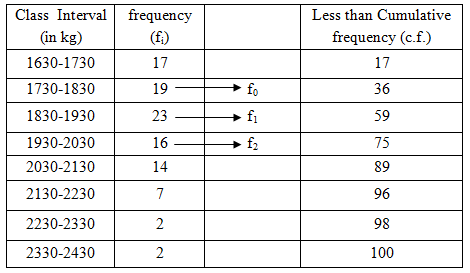
Here N/2=50. Cumulative frequency greater than 50 is 59. Hence the median class is 1830-1930.
![]()
N/4=25. Cumulative frequency greater than 25 is 36. Hence the first quartile class is 1730-1830.
Q1 = 1730 + (25-17) × ![]() =
1730 + 42.1053 = 1772.1053
=
1730 + 42.1053 = 1772.1053
3N/4=75. Cumulative frequency greater than 75 is 89. Hence the third quartile class is 2030-2130.
![]()
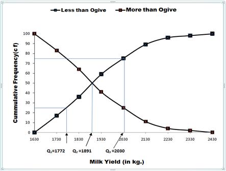
Fig. 3.1 Graphical method to find first quartile, median and third quartile
For computing Mode, the maximum frequency (23) occurs in the class interval 1830-1930, which is called modal class.f1=23, f0=19 and f2=16. Using formula
![]()
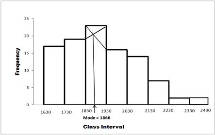
Fig. 3.2 Graphical method to find mode
Empirical relation between Mean, Median and Mode
In
case of symmetrical distribution mean, mode and median coincide while for
asymmetrical distribution the empirical relationship is Mode = 3 Median -2
Mean.