Module 1. Descriptive statistics
Lesson 5
MEASURES OF SKEWNESS AND KURTOSIS
5.1 Introduction
In the preceding lessons, we have discussed the measures of central tendency and dispersion in case of frequency distribution. The measures of central tendency tell us about the concentration of the observations about the middle of the distribution and the measure of dispersion gives us an idea about the spread or scatter of the observations about some measure of central tendency. These measures, however, don’t adequately describe a frequency distribution in the sense that there could be two or more distributions with the same mean and standard deviation but still different from each other with regard to shape or pattern of distribution. Thus these two measures of central tendency and dispersion are inadequate to characterize a distribution completely and must be supported and supplemented by two more measures viz. skewness and kurtosis which we shall discuss in this lesson.
5.2 Skewness
Literal meaning of skewness is “lack of symmetry”. It measures the degree of departure of a distribution from symmetry and reveals the direction of scatterdness of the items.
A frequency distribution is said to be symmetrical when values of the variables equidistant from their mean have equal frequencies. If a frequency distribution is not symmetrical, it is said to be asymmetrical or skewed. Any deviation from symmetry is called skewness.
According to Morris Humberg “Skewness refers to the asymmetry or lack of symmetry in the shape of a frequency distribution”.
According to Croxton & Cowden “When a series is not symmetrical it is said to be asymmetrical or skewed”.
According to Simpson & Kafka “Measures of skewness tell us the direction and the extent of skewness. In a symmetrical distribution the mean, median and mode are identical. The more we move away from the mode, the larger the asymmetry or skewness”.
In the words of Riggleman and Frisbee “Skewness is the lack of symmetry when a frequency distribution is plotted on a chart, skewness present in the items tends to be dispersed more on one side of the mean than on the other”.
Thus the above definitions make it clear that the word skewness refers to the lack of symmetry. If a distribution is normal there would be no skewness in it and the curve drawn from the distribution would be symmetrical. In case of skewed distributions the curve drawn would be elongated either to the left or to the right. The concept of skewness gains importance from the fact that statistical theory is often based upon the assumption of the normal distribution. A measure of skewness is, therefore necessary in order to guard against the consequences of the assumption. The following three figures would give an idea about the shape of symmetrical and asymmetrical curves.
5.2.1 Symmetrical curve
The figure 5.1, given below, presents the shape of a symmetrical curve which is bell shaped having no skewness. The value of mean (M), median (Md) and mode (Mo) for such a curve would be identical.

Fig. 5.1 Symmetrical distribution
In a symmetrical distribution the values of mean, median and mode coincide. The spread of the frequencies is the same on both sides of the centre point of the curve. For a symmetrical distribution Mean = Median = Mode.
5.2.2 Positively skewed curve
A positively skewed curve has a longer tail towards the higher values of X i.e. the frequency curve gradually slopes down towards the higher values of X. In a positively skewed distribution the mean is greater than the median and then mode and the median lies in between mean and mode. The frequencies are spread over a greater range of values on the high value end of the curve (the right hand side) as is clear from the Fig 5.2.

Fig. 5.2 Positively skewed distribution
For a positively skewed distribution Mean > Median > Mode.
5.2.3 Negatively skewed curve
A negatively skewed curve has a longer tail towards the lower values of X i.e. the frequency curve gradually slopes down towards the lower values of X as shown in Fig. 5.3.

Fig. 5.3 Negatively skewed distribution
In the negatively skewed distribution the mode is the maximum and mean is the least. The median lies in between mean and mode. The elongated tail in negatively skewed distribution is on the left hand side as would be clear from Fig 5.3. For a negatively skewed distribution, Mean < Median < Mode.
5.3 Measures of Skewness
Measures of skewness are meant to give an idea about the extent of asymmetry in a series. A distribution is said to be skewed if
· The frequency curve of the distribution is not a symmetric bell shaped curve but stretched more to one side than to the other.
· The values of mean (M), median (Md) and mode (Mo) fall at different points i.e they don’t coincide.
· Quartiles Q1 and Q3 are not equidistant from the median.
· The corresponding pairs of deciles and percentiles are not equidistant from the median.
If a particular distribution is found to be skewed, the next problem that arises is to measure the extent of skewness. To find out the direction and extent of asymmetry in a series statistical measures of skewness are employed.
These measures can be absolute or relative. The absolute measures of skewness tell us the extent of asymmetry and whether it is positive or negative. The absolute skewness is based on the difference between mean and mode. Symbolically,
Absolute skewness = Mean – Mode
Skewness will be positive, if the value of mean is greater than the mode and skewness will be negative, if the value of mean is less than the mode. The difference between the mean and the mode, whether positive or negative, indicates the distribution is positively skewed or negatively skewed. However, such an absolute measure of skewness is not adequate because it cannot be used for comparison of skewness in two distributions, if they are in different units, since difference between the mean and mode will be in terms of the units of distribution. Thus for comparison purposes we use the relative measures of skewness known as co-efficient of skewness.
5.3.1 Karl pearson’s coefficient of skewness
The first
coefficient of skewness as defined by Karl Pearson is
![]()
This measure is
based on the fact that the mean and the mode are drawn widely apart. Skewness
will be positive if mean > mode and negative if mean < mode. There is no
limit to this measure in theory and this is a slight drawback. But in practice
the value given by this formula is rarely very high and its value usually lies
between -1 and +1.
It may also be
written as ![]() as Mode = 3 Median – 2 Mean
as Mode = 3 Median – 2 Mean
This coefficient is a pure number without units since both numerator and denominator have the same dimensions. The value of this coefficient lies between -3 and +3.
5.3.2 Bowley’s Coefficient of Skewness
Prof. A.L. Bowley’s Coefficient of
Skewness is based on quartiles and is given by:
![]()
This is also known as Coefficient of Skewness based on quartiles and is especially useful in situations where quartiles and median are used viz.
· When the mode is ill-defined and extreme observations are present in the data.
· When the distribution has open end classes or unequal class intervals.
This coefficient is a pure number without units since both numerator and denominator have the same dimensions. The value of this coefficient lies between -1 and +1.
5.3.3 Kelly’s Coefficient of Skewness
The
drawback of Bowley’s Coefficient of Skewness is that it ignores the 50% of the
data which can be partially removed by taking two deciles or percentiles
equidistant from the median value. The refinement was suggested by Kelly.
![]()
5.3.4 Coefficient of Skewness based on moments
5.3.4.1 Moments
Moments are the general statistical measure used to describe and analyse the characteristics of a frequency distribution viz. central tendency, dispersion, skewness and kurtosis. Let us consider the variable X having a frequency distribution as given below:
|
X |
X1 |
X2 |
X3 |
---- |
--- |
Xn |
|
f |
f1 |
f2 |
f3 |
---- |
--- |
fn |
Then, ![]() is the arithmetic mean.
is the arithmetic mean.
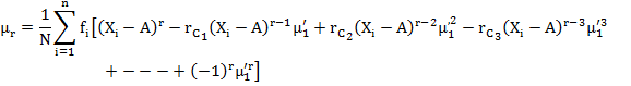
5.3.4.2 Moments about Mean
The
rth moment about Mean ![]() is
denoted by µr and also known as central moment and is defined as
is
denoted by µr and also known as central moment and is defined as
![]() ………(Eq. 5.1)
………(Eq. 5.1)
Putting r=0 in
equation (5.1) we get
![]() ………( Eq. 5.2)
………( Eq. 5.2)
Putting r=1 in equation (5.1) we
get ![]() ………(Eq.
5.3)
………(Eq.
5.3)
because the algebraic sum of deviations of a given set of observations from their mean is zero. Thus the first moment about mean is always zero.
Again taking r=2 we get ![]() ………(Eq.
5.4)
………(Eq.
5.4)
Hence second moment about
mean gives the variance of the distribution.
![]() ………(Eq.
5.5)
………(Eq.
5.5)
![]() ………(Eq. 5.6)
………(Eq. 5.6)
5.3.4.3 Moments about an arbitrary point A
The rth moment about any point A denoted by µr’ are also known as raw moment and is defined as
![]() ………(Eq. 5.7)
………(Eq. 5.7)
Putting r=0 and
r=1 in equation (5.7) we get respectively ![]()
![]() ………(Eq. 5.8)
………(Eq. 5.8)
![]() ………(Eq. 5.9)
………(Eq. 5.9)
![]() where
where ![]() is the first moment about the arbitrary point
A ………(Eq. 5.10)
is the first moment about the arbitrary point
A ………(Eq. 5.10)
Taking r=2, 3, 4 in (5.7) we get respectively
Second moment about the point
A ![]() ………(Eq. 5.11)
………(Eq. 5.11)
Third
moment about the point A ![]() ………(Eq. 5.12)
………(Eq. 5.12)
Fourth
moment about the point A ![]() ………(Eq. 5.13)
………(Eq. 5.13)
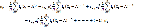
5.3.4.4 Relation between moments about mean and moments about an arbitrary point A
In this section
we shall try to obtain the expression for ![]() ,
the rth moment about mean as defined in (5.1) in terms of
,
the rth moment about mean as defined in (5.1) in terms of ![]() , the rth moment about any
arbitrary point A as defined in (5.7).
, the rth moment about any
arbitrary point A as defined in (5.7).
![]() ………(Eq.
5.14)
………(Eq.
5.14)
From (5.9) we get ![]() , substituting in (5.14) we get
, substituting in (5.14) we get
![]()
Now by binomial theorem
![]()
Putting r = 2, 3, 4 respectively, we get
![]()
![]()
![]()
![]()
![]()
![]()
![]()
![]()
![]()
= ![]()
5.3.4.5 Pearson’s β and γ coefficients
Karl Pearson
gave the following four coefficients calculated from the moments about mean and
defined them as follows:
![]()
These coefficients are pure numbers independent of units of measurement and as such can be conveniently used for comparative studies.
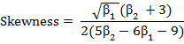
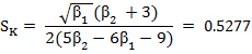
In terms of these coefficients, the coefficient of skewness is given exactly by
The importance of these coefficients lies in the fact that they give some idea about the shape of the curve obtained from the frequency distribution. For symmetrical distribution, all the moments of odd order about the mean vanish or (are zero) and therefore µ3 = 0 and hence β1 = 0. Thus, β1 gives a measure of departure from symmetry i.e. of skewness. Thus, the sign of skewness depends upon µ3. If µ3 is positive we get positive skewness and if µ3 is negative, we get negative skewness.
5.4 Kurtosis
The expression Kurtosis is used to describe the peakedness of a curve. Kurtosis is a Greek word means ‘bulginess’. In statistics kurtosis refers to the degree of flatness or peakedness in the region about the mode of a frequency curve. The degree of Kurtosis of a distribution is measured relative to the peakedness of normal curve. If we know the measures of central tendency, dispersion and skewness, we cannot still form a complete idea about the distribution as is clear from the figure 5.4.
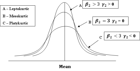
Fig. 5.4 Type of kurtosis
All the three curves are symmetrical about mean and have same variation (range). In order to identify a distribution completely we need one more measure which Prof. Karl Pearson called ‘convexity of the curve’ or ‘kurtosis’. It is measured by β2 and γ2 given as under
![]()
Curve of type B which is neither flat nor peaked is
known as normal curve and shape of its hump is accepted as a standard one.
Curves with humps of the form of normal curve are said to have normal kurtosis
and are termed as Mesokurtic ![]() .The
curve of type A , which are more peaked than the normal curve are known as Leptokurtic
.The
curve of type A , which are more peaked than the normal curve are known as Leptokurtic
![]() and are said to lack kurtosis or to have
negative kurtosis. Curves of type C , which are flatter than the normal curve
are called Platykurtic
and are said to lack kurtosis or to have
negative kurtosis. Curves of type C , which are flatter than the normal curve
are called Platykurtic ![]() and they are said to posses kurtosis in excess
or have positive kurtosis.
and they are said to posses kurtosis in excess
or have positive kurtosis.
Example 1: Find different measures of skewness and kurtosis taking data given in example 1 of Lesson 3, using different methods.
Solution: Prepare the following table to calculate different measures of skewness and kurtosis using the values of Mean (M) = 1910, Median (Md) = 1890.8696, Mode (Mo) = 1866.3636, Variance σ2 = 29500, Q1 = 1772.1053 and Q3 = 2030 as calculated earlier.
Calculation of moments about an arbitrary constant 2080
|
Class Interval |
Mid-value (Xi) |
frequency (fi) |
|
|
|
|
|
|
1630-1730 |
1680 |
17 |
-400 |
-6800 |
2720000 |
-1088000000 |
435200000000 |
|
1730-1830 |
1780 |
19 |
-300 |
-5700 |
1710000 |
-513000000 |
153900000000 |
|
1830-1930 |
1880 |
23 |
-200 |
-4600 |
920000 |
-184000000 |
36800000000 |
|
1930-2030 |
1980 |
16 |
-100 |
-1600 |
160000 |
-16000000 |
1600000000 |
|
2030-2130 |
2080 |
14 |
0 |
0 |
0 |
0 |
0 |
|
2130-2230 |
2180 |
7 |
100 |
700 |
70000 |
7000000 |
700000000 |
|
2230-2330 |
2280 |
2 |
200 |
400 |
80000 |
16000000 |
3200000000 |
|
2330-2430 |
2380 |
2 |
300 |
600 |
180000 |
54000000 |
16200000000 |
|
Total |
|
100 |
-400 |
-17000 |
5840000 |
-1724000000 |
647600000000 |
First moment about the point A=2080

Second moment about the point A
![]()
Third moment
about the point A
![]()
Fourth moment
about the point A
![]()
Compute the central moments using raw moments as
follows:
![]()
![]()
= (-17240000) – 3(58400)(-170) + 2(-170)3
=2718000
![]()
=6476000000 – 4(-17240000)(-170) +
6(58400)(-170)2 – 3(-170)4
= 2373730000
Calculation of moments about mean
|
Class Interval |
Mid-value (Xi) |
frequency (fi) |
|
|
|
|
|
|
1630-1730 |
1680 |
17 |
-230 |
-3910 |
899300 |
-206839000 |
47572970000 |
|
1730-1830 |
1780 |
19 |
-130 |
-2470 |
321100 |
-41743000 |
5426590000 |
|
1830-1930 |
1880 |
23 |
-30 |
-690 |
20700 |
-621000 |
18630000 |
|
1930-2030 |
1980 |
16 |
70 |
1120 |
78400 |
5488000 |
384160000 |
|
2030-2130 |
2080 |
14 |
170 |
2380 |
404600 |
68782000 |
11692940000 |
|
2130-2230 |
2180 |
7 |
270 |
1890 |
510300 |
137781000 |
37200870000 |
|
2230-2330 |
2280 |
2 |
370 |
740 |
273800 |
101306000 |
37483220000 |
|
2330-2430 |
2380 |
2 |
470 |
940 |
441800 |
207646000 |
97593620000 |
|
Total |
|
100 |
|
0 |
2950000 |
271800000 |
237373000000 |
First moment about mean :
![]()
Second moment about mean:
![]() .
.
which is equal to variance as calculated in example 2.
Third moment about mean:
![]()
Fourth moment about mean:
![]()
Karl Pearson’s
Coefficient of skewness (SK):
![]()
Bowley’s Coefficient of skewness (SK):
![]()
From the above calculation the coefficient of skewness and kurtosis can be calculated as under:
![]()
![]()
Hence
this frequency distribution is positively skewed and platykurtic in nature.