Module 3.
Probability distributions
Lesson 10
BINOMIAL DISTRIBUTION
10.1
Introduction
In the first
module we have studied the empirical or observed or experimental frequency
distribution in which the actual data were collected and tabulated in the form
of a frequency distribution. In the present lesson we will study theoretical
frequency distribution which are not obtained by actual observations or
experiments but distributed according to some definite probability law which
can be expressed mathematically. Such distributions as are expected on the
basis of previous experience or theoretical considerations are known as
theoretical distribution or probability distribution. Thus, the theoretical
frequency distribution are not based on actual observations but are
mathematically deducted under certain assumptions. In this lesson we shall
study one of the most popular discrete distributions, the origin of which lies
in Bernoullian trials.
10.2 Binomial
Distribution
Binomial
distribution is a discrete probability distribution. This distribution was
discovered by a Swiss Mathematician James Bernoulli (1654-1705). A Bernoullian
trial is an experiment having only two possible outcomes i.e. success or
failure. In other words the result of the trial are dichotomous e.g. in tossing
of a coin either head or tail, the sex of a calf can be either male or female,
a manufactured milk product or an engineering equipment or spare part will be
either defective or non defective etc. This distribution can be used under the
following conditions:
a) The random experiment is performed repeatedly a finite and fixed number of times i.e. n, the number of trials is finite and fixed.
b) The outcome of a trial results in the dichotomous classification of events i.e. each trial must result in two mutually exclusive outcomes –success or failure.
c) Probability of success (or failure) remains same in each trial i.e. in each trail the probability of success, denoted by p remains constant. q=1-p, is then termed as the probability of failure (non-occurrence).
d) Trials are independent i.e. the outcome of any trial does not affect the outcomes of the subsequent trials.
10.3 Probability Mass Function of Binomial Distribution
Statement
If X denotes the number of successes in n trials satisfying the above conditions, then X is a random variable which can take values 0,1,2,---,n i.e. no success, one success, two successes,---, or all the n successes. The general expression for the probability of r successes is given by:
P(r) = P(X = r) = nCr pr qn-r for r=0,1,2,………,n
Proof : By the theorem of compound probability, the probability that r trials are success and the remaining (n-r) are failures in a sequence of n trials in a specified order say S,F,S,F,S,,---,S is given by

But we are interested in any r trials being successes and since r trials can be chosen out of n trials in nCr (mutually exclusive) ways. Therefore, by the theorem of total probability, the chance P (r) of r successes in a series of n independent trials is given by
P (r) = nCr pr qn-r 0≤r≤n
r can take only positive integer values.
Thus, the chance variate i.e. the number of successes, can take the values 0,1,2,…..,r,……..,n with corresponding probabilities qn,nC1 p qn-1,………..,nCr pr qn-r,………..,pn
o The probability distribution of the number of successes so obtained is called the binomial probability distribution for the obvious reason that the probabilities are the various terms of the binomial expansion of (q+p)n.
o The sum of probabilities
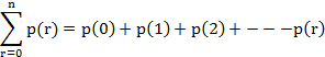
![]()
o
The expression for P (X = r) is known as
probability mass function of the Binomial distribution with parameter n and p.
The random variable X following this probability law is called binomial variate
with parmeter n and p denoted as X~B(n,p).Hence binomial distribution can
be completely determined if n and p are known .
Example 1.
It is known that 40 percent cows affected by tuberculosis die every year. Six
cows are admitted to a veterinary hospital suffering from tuberculosis. What is
the probability that
(i) Three
cows will die.
(ii)
at least five cows will die
(iii) all
cows will be cured
(iv)
no cow will be saved.
Solution
In this exercise we have p = 0.4 , q = 1- 0.40
= 0.6 and n=6
In binomial distribution we have P(r) = nCr
. pr . qn-r
(i) Prob. [Three cows will die] = P[r = 3] = P(3) = 6C3
. (0.4)3 (0.6)3
![]()
(ii) Prob. (at least five cows will die) = P(5) +
P(6) = 6C5 (0.4)5 (0.6)1 + 6C6
(0.4)6 (0.6)0 = 6
(0.4)5 (0.6)1 + (0.4)6 = 0.0369 +0.0041=
0.0410
(iii) Prob. (all cows will be cured) =1
– P (no cow will die) = 1- P(0) =1 – 6C0 (0.4)0
(0.6)6 = 1 - (0.6)6 = 1 – 0.0467 = 0.9533
(iv) Prob. (no cow will be saved) = P
(all cows will die) = P(6)= 6C6 (0.4)6
(0.6)0 = (0.4)6 =0.0041
Example 2. Ten
consumers were asked to state their preferences between two types of ice-cream.
Assuming that there is no difference between two types of ice–cream, calculate
the probability that
a)
3 or less consumers will prefer ice-cream A.
b)
7 or more consumers will prefer ice-cream B.
Solution:
In this exercise p = 0.5, q = 0.5 and n = 10
a) Prob. [Three or
less consumers will prefer Ice Cream A] = P(0) + P(1) + P(2) + P(3)
= 10C0
(0.5)0 (0.5)10 + 10C1 (0.5)1(0.5)9
+ 10C2 (0.5)2 (0.5)8 + 10C3
(0.5)3(0.5)7 = (0.5)10(10C0
+ 10C1 + 10C2 + 10C3)
=
0.00098 (1 + 10+ 45 + 120) = 0.00098 (176) = 0.1725
b) Prob. [Seven or more consumers will
prefer Ice Cream B] = P(7) + P(8) + P(9) + P(10)
= 10C7
(0.5)7 (0.5)3 + 10C8 (0.5)8(0.5)2
+ 10C9 (0.5)9 (0.5)1 + 10C10
(0.5)10 = (120+45+10+1) (0.5)10 =0.1725
10.4
Example of Binomial distribution
·
The problem relating to tossing of a coin or throwing of dice or drawing cards
from a pack of cards with replacement.
·
The problems relating to distribution for the preference for a dairy product
among families.
·
The problem relating to distribution of coli-forms in sterilized milk.
·
The problem relating to distribution of number of stables in farm households.
·
The problem relating to distribution of number of lactations completed by the
milch animals in a dairy farm.
10.5
Properties of Binomial Distribution
i) Mean of
binomial distribution is np.
Proof:
First raw moment
![]()
![]()

ii)
Variance of binomial distribution is npq
Proof:
Second raw moment
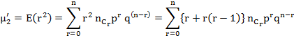

Variance = ![]()
For the binomial distribution if mean and variance are known, we can arrive at the frequency distribution and variance is less than mean.
iii) The third and fourth
central moment µ3 and µ4 can be obtained on the same
lines.
![]()
![]()
iv)
Pearson’s constants β1 & β2 as well as
γ1 and γ2 are given by
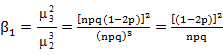
![]()
γ1
shows that the binomial distribution is positively skewed if q > p or p <
1/2 and it is negatively skewed if q < p or p >1/2 and it is symmetrical
if p = q = 1/2.The binomial distribution is leptokurtic if pq < 1/6 and
platykurtic if pq > 1/6.
v) Mode of binomial distribution is determined by the value (n+1)p. If this value is an integer equal to k then the distribution is bi-modal, the two modal values being X=k and X=k-1.When this value is not an integer then the distribution has unique mode at X=k1, the integral part of (n+1)p.
vi) Additive property: If X1 is B(n1,p)and X2 is B(n2,p) and they are independent then their sum X1 + X2 is also a binomial variate B(n1+ n2,p).
Example
3.
If the mean and variance of a Binomial Distribution are respectively 9 and 6,
find the distribution.
Solution:
Mean
of Binomial Distribution is np and variance is npq
![]()
![]()
![]()
![]()
Hence,
the Binomial Distribution is ![]()
i.e.
![]()
Example
4. An unbiased dice is thrown 5 times and appearance of face on the dice 2
or 3 is considered as success. Find the probability of (i) exactly one success
(ii) at least 4 successes and find mean and variance.
Solution:
Here ![]()
![]()
![]()
![]()
![]()
![]()
![]()
![]()
Example 5.
A binomial variate X satisfies the relation 9 P(X=4)=P(X=2) when n = 6. Find
the value of the parameter p.
Solution:
Since the binomial probability distribution is
![]()
![]()
![]()
Considering
the given relation,
9 P(X = 4) = P(X = 2), we have
![]()
![]()
![]()
![]() .
.
10.6 Fitting of Binomial Distribution
Let the n independent trials constitute one experiment and let this experiment be repeated N times. Then we expect r successes to occur N. nCr pr qn-r times. This is called expected frequency of r successes in N experiments and the possible number of successes together with the expected frequencies will constitute binomial (expected) frequency distribution
Nxp(r)
= Nx nCr pr qn-r ;![]() r=0,1,2,………,n
r=0,1,2,………,n
Putting r=0,1,2,………,n we get the expected or theoretical frequencies of the Binomial distribution , which are given in the following table .
|
No. of successes ( r ) |
Expected or theoretical Frequencies N.P(r) |
|
0 |
N |
|
1 |
N |
|
2 |
N |
|
: |
: |
|
n |
N |
Case I: If p the probability of success which is constant for each trial is known , then the expected frequencies can be obtained from the above table.
Case II: If p is not known and
if we want to fit a binomial distribution to a given frequency distribution,
then first find mean of the given frequency distribution by the formula ![]() and equate it to np which is mean of the
binomial distribution. Hence, p can be estimated by the relation m=np⇒p=m/n, q = 1-p, with
the values of p and q the expected theoretical binomial frequencies can be
obtained by using the above table. The expected frequencies can also be
computed by using the following recurrence formula
and equate it to np which is mean of the
binomial distribution. Hence, p can be estimated by the relation m=np⇒p=m/n, q = 1-p, with
the values of p and q the expected theoretical binomial frequencies can be
obtained by using the above table. The expected frequencies can also be
computed by using the following recurrence formula
![]()
The procedure is illustrated through the following example.
Example 6. The following table gives the number of coliforms per ml in thousand pouches of milk:
|
No of coliforms (Xi) |
0 |
1 |
2 |
3 |
4 |
5 |
6 |
7 |
8 |
9 |
10 |
|
No. of pouches (fi) |
2 |
8 |
46 |
116 |
211 |
243 |
208 |
119 |
40 |
7 |
0 |
Fit a binomial distribution to the above data.
Solution: In the usual
notations we have: n = 10, N = 1000, ∑
fi Xi = 4971,
![]()
![]()
to get the expected frequencies as given in the following table:
|
No. of coliforms (Xi) |
No. of bottles (fi) |
fi Xi |
Expected Frequency E (r) |
|
0 |
2 |
0 |
1.0347 |
|
1 |
8 |
8 |
10.2277 |
|
2 |
46 |
92 |
45.4939 |
|
3 |
116 |
348 |
119.9179 |
|
4 |
211 |
844 |
207.4360 |
|
5 |
243 |
1215 |
246.0524 |
|
6 |
208 |
1248 |
202.6788 |
|
7 |
119 |
833 |
114.4808 |
|
8 |
40 |
320 |
42.4352 |
|
9 |
7 |
63 |
9.3213 |
|
10 |
0 |
0 |
0.9214 |
|
Total |
1000 |
4971 |
1000.00 |
Different expected frequencies are also computed by using recurrence formula
![]()
![]()
![]()
![]()
![]()
![]()