Module 3.
Probability distributions
Lesson 12
NORMAL DISTRIBUTION
12.1
Introduction
In preceding two
lessons discrete probability distributions viz., Binomial and Poisson
distribution were discussed. We shall now take up another distribution, which
is an important continuous probability distribution known as the normal
distribution. Normal distribution is probably the most important and widely
used theoretical distribution. Normal distribution unlike the Binomial and
Poisson is a continuous probability distribution. It has been observed that a
vast number of variables arising in studies of agricultural and dairying,
social, psychological and economic phenomena tend to follow normal
distribution. The normal distribution was first discovered by French Mathematician
Abraham De-Moivre in 1733, who obtained this continuous distribution as a
limiting case of the Binomial distribution. But it was later rediscovered and
applied by Laplace and Karl Gauss. It is also known as Gaussian distribution
after the name of Karl Friedrich Gauss.
12.2 Definition of Normal
Distribution
A
continuous random variable X is said to have a normal distribution with
parameters µ (mean) and σ (standard deviation), if its density function is
given by the probability law
![]()
where
π and e are given by π = 22/7 and e=2.7183 (base of natural
logarithms).
Remarks
1) A
random variable X with mean µ and variance σ 2 following the
normal law given above is represented as X~N(µ, σ 2).
2) If
X~N(µ, σ 2) , then ![]() , is defined as a standard normal variate with
E(Z)=0 and Var (Z)=1and we write Z~N(0, 1)
, is defined as a standard normal variate with
E(Z)=0 and Var (Z)=1and we write Z~N(0, 1)
3) The
p.d.f. of a standard normal variate Z is given by
![]()
4) Normal
distribution is a limiting form of the binomial distribution when
a)
n, the number of trials is indefinite large, i.e. n→∞ and
b) neither
p nor q is very small.
5)
Normal distribution is a limiting form of Poisson distribution when its mean m
is large and n is also large.
12.3 Chief Characteristics
(Properties) of Normal Distribution
It has the following properties:
1. The
graph of f(x) is bell shaped unimodal and symmetric curve as shown in the Fig.
12.1. The top of the bell is directly above the mean (µ).
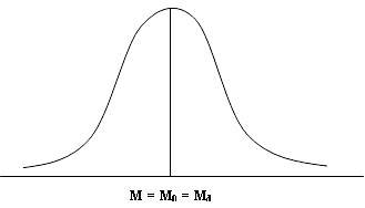
Fig.
12.1 Normal probability curve
2. The
curve is symmetrical about the line X = μ, (Z = 0) i.e., it has the same
shape on either side of the line X = μ, (or Z = 0). This is because the
equation of the curve ∅(z)
remains unchanged if we change z to -z.
3. Since
the distribution is symmetrical, mean, median and mode coincide. Thus, Mean =
Median = Mode = μ
4. Since
Mean = Median = Mode = μ, the ordinate at X = μ, (Z = 0) divides the
whole area into two equal parts. Further, since total area under normal
probability curve is 1, the area to the right of the ordinate as well as to the
left of the ordinate at X = μ (or Z = 0) is 0.5
5. Also,
by virtue of symmetry the quartiles are equidistant from median (µ), i.e,
![]()
6. Since
the distribution is symmetrical, all moments of odd order about the mean are
zero. Thus μ2n+1 = 0; (n = 0,1,2,…) i.e. μ1 = μ3 =
μ5 = --- = 0.
7. The
moments (about mean) of even order are given by
![]()
Putting n=1 and 2 we
get
μ2
= σ2 and μ4 = 3σ4
![]()
and
![]()
8. Since
the distribution is symmetrical, the moment coefficient of skewness based on
moments is given by
![]()
9. The
coefficient of kurtosis is given by
![]()
10. No
portion of the curve lies below the x-axis, since f(x) being the probability
can never be negative.
11. Theoretically,
the range of the distribution is from -∞ < to < ∞. But
practically, range = 6σ
12.
As x increases numerically [i.e. on either side of X = μ], the value of
f(x) decreases rapidly, the maximum probability occurring at X = μ and is
given by
![]()
Thus maximum value of
f(x) is inversely proportional to the standard deviation. For large values of
σ, f(x) increases, i.e., the curve has a normal peak.
13.
Distribution is unimodal with the only mode occurring at X =
μ.
14. X-axis
is an asymptote to the curve i.e., for numerically large value of X (on either
side of the line (X = μ)), the curve becomes parallel to the X-axis
and is supposed to meet it at infinity.
15. A
linear combination of independent normal variates is also a normal variate. If
X1,X2, … ,Xn are independent normal variates
with mean μ1,μ2, … ,μn and
standard deviations σ1, σ2, … ,
σn respectively then their linear combination
![]()
Where a1, a2, … , an
are constants, is also a normal variate with Mean = a1μ1+
a2μ2 + … + an μn and
Variance = a12 σ12 + a22
σ22 + … + an2 σn2.
In particular, if we take a1 = a2 = … = an =1
then we get “X1+X2 + … +Xn is a normal variate
with mean μ1+μ2+ … +μn and
variance σ12 + σ22 + … +
σn2 “.Thus, the sum of independent normal variates
is also a normal variate with mean equal to sum of their means and standard
deviation equal to square root of sum of the squares of their standard
deviations. This is known as the ‘Re-productive or Additive Property’ of the
Normal distribution.
16. Mean
Deviation (M.D.) about mean or median or mode is given by
17. Quartiles
are given (in terms of µ and σ) by
![]()
18. Quartile
deviation (Q.D.) is given by
![]()
Also
![]()
![]()
19. We
have (approximately):
![]()
From property 18 we also have ![]()
20. Points
of inflexion of the normal curve are at X = μ ± σ i.e. they are
equidistant from mean at a distance of σ and are given by :
![]() ,
,![]()
21. Area
property: One of the most fundamental property of the normal probability curve
is the area property. If X ∽ N (µ, σ2),
then the probability that random value of X will lie between X= μ and X= x1 is given
![]()

∴
P (µ < x < x1) = P (0 < z < z1)
![]()
Where ![]() is the probability function of standard normal
variate. The definite integral
is the probability function of standard normal
variate. The definite integral ![]() is known as Normal Probability integral
and gives the area under standard normal curve between the ordinate z=0 and z =
z1. These areas have been provided in the form of table for
different values of z1 at the intervals of 0.01 which are available
in any standard text books of statistics.
is known as Normal Probability integral
and gives the area under standard normal curve between the ordinate z=0 and z =
z1. These areas have been provided in the form of table for
different values of z1 at the intervals of 0.01 which are available
in any standard text books of statistics.
Particular
Cases:
1. In
particular, the probability that a random variable X lies in the interval
(μ-σ, μ+σ) is given by
![]()
![]()
The area under
the normal probability curve between the ordinates at X= μ-σ and X= μ+σ is 0.6826.In other
words, the range X = μ±σ covers 68.26% of the observations (as
shown in Fig.12.2). This is known as 1σ limit of normal distribution
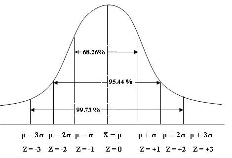
Fig.
12.2 1σ, 2σ and 3σ under Normal Probability Curve
2.
The probability that random variable X lies in the interval (μ-2σ,
μ+2σ) is given by
![]()
![]()
The area under the normal probability
curve between the ordinates at X=
μ-2σ and X= μ+2σ is
0.95445. In other words, the range X = μ±2σ covers 95.445% of the
observations (as shown in Fig. 12.2). This is known as 2σ limits of normal
distribution and is considered as warning limit in case of statistical quality
control which implies that it is a warning to the manufacturer that the
manufacturing process is going out of control.
3.
The probability that random variable X lies in the interval (μ−3σ,
μ+3σ) is given by
![]()
![]()
The
area under the normal probability curve between the ordinates at X=μ−3σ and X= μ+3σ is 0.9973.In other words, the range X = μ±2σ covers
99.73% of the observations (as shown in Fig. 12.2). This is known as 3σ
limits of normal distribution and it implies the manufacturing process is out
of control in case of statistical quality control.
Thus, the probability that a normal
variate X lies outside the range µ ± 3σ is given as
![]()
Thus, in all probability, we should
expect a normal variate to lie within the range µ ± 3σ though
theoretically may range from −∞ to ∞.
12.4
Examples of Normal Distribution
(i)
The age at first calving of cows belonging to the same breed and living under
similar environmental conditions tend to normal frequency distribution.
(ii)
The milk yield of cows in a large herd tends to follow a normal frequency
distribution.
(iii) The
chemical constituents of milk like fat, SNF, protein etc. for large samples
follow normal distribution.
12.5 Computation of Area
Under Normal Probability Curve
Probability that a continuous random variable X in
any value between a and b is
![]()
which is the area bounded by the
curve p(x), X-axis and the ordinates at X=a and X=b and is shown in Fig. 12.3.
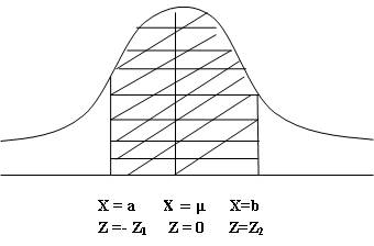
Fig. 12.3
Similarly the area to the right of the
ordinates at X=x1 and x1is less than mean (as shown in
Fig. 12.4 )
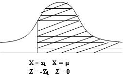
Fig.
12.4
At X=X1 Z=-Z1 so
P(X>X1)=0.5+P(-Z1<Z<0)=0.5+ P(0<Z<Z1)
, where P(0<Z<Z1)can be read from the normal tables. The application
of this distribution in solving problems is illustrated through following
examples.
Example 1.
Average lactation yield for 1000 cows maintained at a farm is 1700 kg and their
standard deviation is 85 kg. A cow is considered as high yielder if it has a
lactation yield greater than 1900 kg and poor yielder if it has lactation yield
less than 1600 kg. Find the number of high yielding and poor yielding cows.
Solution:
Here,
µ=1700 kg and σ = 85 kg and let X denote the lactation milk yield
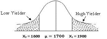
Fig. 12.5
a) To find number of high
yielder cows we first find the probability of cows yielding more than 1900 kg.
i.e. P(X > 1900 kg) (Fig. 12.5). So, we first compute the value
standard normal variate i.e. Z1 and then find area under
shaded region using normal tables
At X1 = 1900 kg.![]()
P(X1 > 1900 kg) = P (Z1
>2.353) =0.5 – P (0≤ Z1 ≤ 2.353) =
0.5–0.49069=0.00931
Number of high
yielder cows = N xP(z1 > 2.353) = 0.00931 ×1000 = 9.31 = 9 cows
b) To find number of low yielder
cows, we first find the probability of cows yielding less than 1600 kg i.e. P(X2
< 1600 kg). So, we first compute the value standard normal variate i.e. Z2
and then find area under shaded region using normal tables ![]()
P(X2
< 1600) = P (Z2 < -1.18)=0.5 – P(0≤ Z2 ≤
1.18) = 0.5–0.38109=0.119
Number
of low yielder cows = N xP(X2 < 1600) = 0.119 × 1000 = 119 cows
Conclusion: Total number of high
yielding & low yielding cows are 9 and 119 respectively.
Example 2.
An Intelligence test was administrated to 1000 students. The average score of
students was 42 with standard
deviation of 24. Find
(a)
Number of students exceeding a score of 50
(b)
Number of students scoring between 30 & 58
(c) Value of score exceeded
by top 100 students.
Solution: In
this problem µ=42 and σ = 24 and let X denote the score obtained
(a) Number of
students exceeding score 50
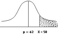
Fig.
12.6
As shown in figure 12.6 we want to
find P(X>50) i.e. probability of shaded portion
At
X=50, ![]()
P(X>50)
=P(Z > 0.334) = 0.5 – P(0≤ Z ≤ 0.334)= 0.5 – 0.1308== 0.3692
No of students = 1000 * 0.3692=
369.2 ~ 369 students
(b)
Number of students scoring between 30 and 58
As shown in figure 12.7 we want to find
P(30<X<58) i.e. probability of shaded portion
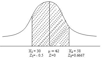
Fig.
12.7
![]()
P(
Z1> -0.5) = P(0≤Z1 ≤ 0.5)= 0.1915
![]()
P(Z2<0.6667)=
P(0 ≤ Z2 ≤ 0.6667)=0.2476
P(30<X<58)=P(-0.5≤
Z≤0.6667) =0.1915+0.2476=0.4391
No of students = 1000 * .4391 = 439.1 ~ 439 students
(c)
Value of score exceeded by top 100 students. Let x1 be the value of
score exceeded by top 100 students, the probability of top 100 students = 100/N
= 100/1000 = 0.1 such that P(X>x1) = 0.1
At
X= x1 , ![]() =
Z1 . From Fig. 12.8 the P(X>x1) shown as shaded region
=
Z1 . From Fig. 12.8 the P(X>x1) shown as shaded region
P(X>x1)=P(Z>Z1)=0.1 ⇒P(0
≤ Z ≤ Z1)=0.4 ![]() =
1.286
=
1.286
x1=
72.86 ~73
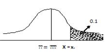
Fig.
12.8
Conclusion
(a) 369 students scored
more than 50.
(b) 439 students scored
between 30 & 58.
(c) Minimum score of
top 100 students is 73.
Example 3.
Tins are filled by an automatic filling machine with ghee. Average
quantity filled in tin is 1000g. It is found that 5% of tins had ghee less than
980 grams. Find the standard deviation.
Solution :
Here µ=1000g and let X be quantity of ghee filled in a tin
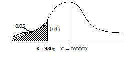
Fig.
12.9
From fig. 12.9 P(X
<980)=0.05 ⇒
P(Z < -Z1) = -1.645
⇒
(980-1000/σ) -1.645 ⇒ -20 = -1.645
σ , Hence σ =12.1840~12.18 gm
Conclusion :
Standard derivation of the ghee filled in tin is
12.18 gm.
Example 4.
In a normal distribution, 31% of items are under 45 and 8% are over 64.
Find the mean & standard deviation.
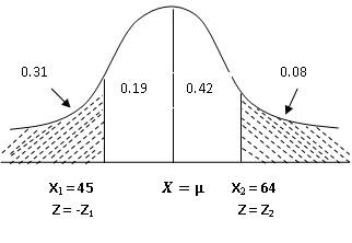
Fig.
12.10
Solution:
Let
X denotes the variable under consideration. We are given that P (X1 <
45) = 0.31 and P (X2 > 64) = 0.08. If X has normal distribution
with mean µ and standard deviation σ. Then standard normal variates
corresponding to X1 = 45 and X2 = 64 (from Fig 12.10) are
When
X1 = 45, ![]()
When
X2 = 64, ![]()
From
the fig. 12.10, P (0 <Z < Z2) = 0.42 ⇒
Z2 = 1.405 (from normal tables)
![]() .........(Eq. 1)
.........(Eq. 1)
P
(-Z1 <Z < 0) = 0.19 ⇒
P (0 <Z < Z1) = -0.496 (from normal tables)
![]() .........(Eq.
2)
.........(Eq.
2)
Solving
equations (1) & (2) we get
μ=
49.95 ~ 50 and σ = 9.99 ~ 10
Conclusion
Mean
& standard deviation of given distribution are 50 & 10 respectively.
Example 5.
Average net weight
of coffee complete powder is 250 g with a standard deviation of 3g. The powder
is packed in polypack with an average weight of 5g with a standard deviation of
0.2g. Average weight of tin in which polypack is packed is 100g with a standard
deviation of 1.5g. Individual weights of all items follow normal distribution.
If 5% tins are classified as underweight tins then what would be the weight of
filled in tin. Filled in tins are classified as overweight if their weight
exceeds a weight of 360g. What proportion of tins are overweight tin?
Solution:
Let X1
be the normal variate for weight of coffee with mean(μ1)=
250g and s.d.(σ1)=3g
X2
be the normal variate for poly pack with mean ( μ2)= 5g
and s.d.(σ2)=0.2 g
X3
be the normal variate for tin with mean (μ3)= 100g and
s.d.(σ3)=1.5 g
By
using the reproductive property of normal distribution, the composite weight of
tin comprising of coffee complete, polypack and tin will follow a normal
distribution with mean (μ=μ1+μ2+μ3)=250+5+100=355g
and standard deviation (![]() ) =
) =![]() =
=![]()
=3.36
g i.e. (X=X1+ X2+ X3)~N(355g,3.36 g) If 5% tins
are classified as underweight, Let x1 be the weight of tin
considered as underweight, then we have : P(X<x1)=0.05. Then the
standard normal variate corresponding to x1 is ![]()
From
fig.12.11 P(−Z1< Z < 0)=0.45⇒P(0<Z<
Z1) = 0.45 ⇒ (x1-355)/3.36
= -1.6415 ⇒ x1 = 349.67g
Hence weight of underweight tins is 349.47 g.
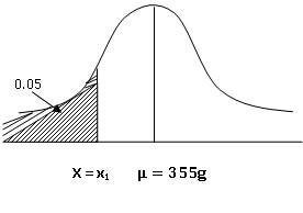
Fig.
12.11
Filled in tins
exceeding a weight of 360g are classified as overweight. To find the proportion
of tins which are overweight we proceed as follows:
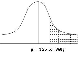
Fig.
12.12
As shown in figure 12.12, we want to find
P(X>360) i.e. probability of shaded portion
At
X=360, ![]()
P
(X > 360) = P (Z > 1.488) = 0.5 – P (0≤ Z ≤ 1.488) = 0.5 –
0.4316== 0.0684
Hence, 6.84 % tins are overweight
Conclusion:
Weight of underweight tins is 349.47g & 6.84%
tins are overweight
12.6
Importance of Normal Distribution
Normal distribution plays a very
important role in statistics because
(i) Most
of the discrete probability distributions occurring in practice e.g., Binomial
and Poisson can be approximated to normal distribution as n number of trials
tends to increase.
(ii) Even if a
variable is not normally distributed, it can be sometimes be brought to normal
by a simple mathematical transformation, if the distribution of X is skewed,
the distribution of ![]() or log x might come out to be normal.
or log x might come out to be normal.
(iii) If
X~N(μ,σ2) then P [μ−3σ < x <
μ+3σ] =0.9973 ⇒ [|Z|˃3] = 1−
0.9973=0.0027. Thus the probability of standard normal variate going outside
the limits ±3 is practically
zero. This property of normal distribution forms the basis of entire large
sample theory.
(iv) Many of the
sampling distribution e.g., student’s t, Snedecor’s F, Chi square distributions
etc tend to normality for large samples. Further, the proof of all the tests of
significance in the sample is based upon the fundamental assumptions that the
populations from which the samples have been drawn are normal.
(v) The
whole theory of exact sample (small sample) tests viz. t , χ2,
F etc, is based on the fundamental assumption that the parent population from
which the samples have been drawn follows normal distribution.
(vi) Normal
distribution finds large applications in statistical quality control in
industry for setting up of control limits.
(vii) Theory of normal curves can
be applied to the graduation of the curve which is not normal.