Module 5. Test of significance

 Lesson 16

TESTING OF HYPOTHESIS

16.1  Introduction

A researcher or experimenter has always some fixed ideas about certain population(s) vis-à-vis population parameters(s) based on prior experiments/sample surveys or past experience. It is therefore desirable to ascertain whether these ideas or claims are correct or not by collecting information in the form of data through conduct of experiment or survey. In this manner, we come across two types of problems, first is to draw inferences about the population on the basis of sample data and other is to decide whether our sample observations have come from a postulated population or not. In this lesson we would be dealing with the second type of problem. In the ensuing section we would provide concepts and definitions of various terms used in connection with the testing of hypothesis.

16.2 Testing of Hypothesis

The inductive inference is based on deciding about the characteristics of the population on the basis of a sample. Such decisions involve an element of risk, the risk of wrong decisions. In this endeavor, modern theory of probability plays an important role in decision making and the branch of statistics which helps us in arriving at the criterion for such decisions is known as testing of hypothesis. The theory of testing of hypothesis was initiated by J. Neyman and E.S. Pearson. Thus, theory of testing of hypothesis employs various statistical techniques to arrive at such decisions on the basis of the sample theory. We first explain some fundamental concepts associated with testing of hypothesis.

16.3  Basic Concepts of Testing of Hypothesis

16.3.1  Hypothesis

According to Webster Hypothesis is defined as tentative theory or supposition provisionally adopted, explain certain facts and guide in the investigation of others e.g. looking at the cloudy weather, the statement that “It may rain today” is considered as hypothesis.

16.3.2 Statistical hypothesis

A statistical hypothesis is some assumption or statement, which may or may not be true about a population, which we want to test on the basis of evidence from a random sample. It is a definite statement about population parameter. In other words, it is a tentative conclusion logically drawn concerning any parameter of the population. For example, the average fat percentage of milk of Red Sindhi Cow is 5%, the average quantity of milk filled in the pouches by an automatic machine is 500 ml.

16.3.3  Null hypothesis

According to Prof. R. A. Fisher “A hypothesis which is tested for possible rejection under the assumption that it is true is usually called Null Hypothesis” and is denoted by H₀.The common way of stating a hypothesis is that there is no difference between the two values, namely the population mean and the sample mean. The term ‘no difference’ means that the difference, if any, is merely due to sampling fluctuations. Thus, if the statistical test shows that the difference is significant, the hypothesis is rejected. A statistical hypothesis which is stated for the purpose of possible acceptance is called Null Hypothesis. To test whether there is any difference between the two populations we shall assume that there is no difference. Similarly, to test whether there is relationship between two variates, we assume there is no relationship. So a hypothesis is an assumption concerning the parameter of the population. The reason is that a hypothesis can be rejected but cannot be proved. Rejection of no difference will mean a difference, while rejection of no relationship will imply a relationship. For example if we want to test that the average milk production of Karan Swiss cows in a lactation is 3000 litres then  the null hypothesis may be expressed symbolically as  H_o: μ = 3000 litres.

16.3.4  Alternative hypothesis

Any hypothesis which is complementary to the null Hypothesis is called an alternative hypothesis. It is usually denoted by H₁ or H_A. For example if we want to test the null hypothesis that the population has a specified mean μ_o  i.e.  H_o: μ=μ_o then the alternative hypothesis could be

(i) H₁: μ ≠ μ_o (μ > μ_o or μ < μ_o)

(ii) H₁: μ > μ_o

(iii) H₁: μ < μ_o

The alternative hypothesis in (i) is known as two tailed alternative and the alternatives in (ii) and (iii) are known as right tailed and left tailed alternatives. The setting of alternative hypothesis is very important since it enables us to decide whether to use a single tailed (right or left) or two tailed test. The null hypothesis consists of only a single parameter value and is usually simple while alternative hypothesis is usually composite.

16.3.5  Simple and composite hypothesis

If the statistical hypothesis completely specifies the population or distribution, it is called a simple hypothesis, otherwise it is called a composite hypothesis. For example, if we consider a normal population N (µ, σ²) where σ² is known and we want to test the hypothesis H₀: µ=25 against H₁: µ=30. From these hypotheses, we know that µ can take either of the two values, 25 or 30. In this case H₀ and H₁ are both simple. But generally H₁ is composite, i.e., of the form H₁: µ≠25, viz, H₁: µ<25 or H₁: µ>25. In sampling from a normal population N (μ, σ²), the hypothesis H: μ=μ₀ and σ²=σ₀² is a simple hypothesis because it completely specifies the distribution. On the other hand (i) μ=μ₀ (σ² is not specified) (ii) σ²=σ₀²  (μ is not specified) (iii) μ<μ_0, σ²=σ₀² etc. are composite hypothesis.

16.3.6  Types of errors in testing of hypothesis

The main objective in sampling theory is to draw a valid inference about the population parameters on the basis of the sample results. In practice we decide to accept or reject a null hypothesis (H₀) after examining a sample from it.  As such we are liable to commit errors. The four possible situations that arise in testing of hypothesis are expressed in the following dichotomous table:

Table 16.1

Decision from sample	True Situation
	Hypothesis is true	Hypothesis is false
Accept the hypothesis	No error	Type II error
Reject the hypothesis	Type I error	No error

In testing hypothesis, there are two possible types of errors which can be made. The error of rejection of a hypothesis H₀ when H₀ is true is known as Type I error and error of acceptance of a hypothesis H₀ when H₀ is false is known as type II error. When setting up an experiment to test a hypothesis it is desirable to minimize the probabilities of making these errors. But practically it is not possible to minimize both these errors simultaneously. In practice, in most decision making problems, it is more risky to accept a wrong hypothesis than to reject a correct one. These two types of errors can be better understood with an example where a patient is given a medicine to cure some disease and his condition is examined for some time. It is just possible that the medicine has a positive effect but it is considered that it has no effect or adverse effect. Therefore it is the Type I error. On the other hand if the medicine has an adverse effect but it is considered to have had a positive effect, it is called Type II error. Now let us consider the implications of these two types of error. If type I error is committed, the patient will be given another medicine, which may or may not be effective. But if type II error is committed i.e., the medicine is continued inspite of an adverse effect, the patient may develop some other complications or may even die. This clearly shows that the type II error is much more serious than the type I error. Hence in drawing inference about the null hypothesis, generally type II error is minimized even at the risk of committing type I error which is usually chosen as 5 per cent or 1 per cent.

Probability of committing type I error and type II error are denoted by α and β and are called size of type I and type II error respectively. In Industrial Quality Control, while inspecting the quality of a manufactured lot, the Type I error and type II error amounts to rejecting a good lot and accepting a bad lot respectively. Hence α=P(Rejecting a good lot) and β=P( Accepting a bad lot). The sizes of type I and type II errors are also known as producer’s risk and consumer’s risk respectively. The value of (1-β) is known as the power of the test.

16.3.7  Level of significance

It is the amount of risk of the type I error which a researcher is ready to tolerate in making a decision about H₀. In other words, it is the maximum size of type I error, which we are prepared to tolerate is called the level of significance. The level of significance denoted by α is conventionally chosen as 0.05 or 0.01. The level of 0.01 is chosen for high precision and the level 0.05 for moderate precision. Sometimes this level of risk is further brought down in medical statistics where the efficiency of life saving drug on the patient is tested. If we adopt 5% level of significance, it means that on 5 out of 100 occasions, we are likely to reject a correct H₀ .In other words this implies that we are 95% confident that our decision to reject H_o is correct_. . That is, we want to make the significance level as small as possible in order to protect the null hypothesis and to prevent, as far as possible, the investigator from inadvertently making false claims. Level of significance is always fixed in advance before collecting the sample information.

16.3.8  P-value concept

Another approach followed in testing of hypothesis is to find out the P-value at which H₀ is significant i.e., to find the smallest level α at which H₀ is rejected. In this situation, it is not inferred whether H₀ is accepted or rejected at a level of 0.05 or 0.01 or any other level. But the researcher only gives the smallest level α at which H₀ is rejected. This facilitates an individual to decide for himself as to how much significant the research results are. This approach avoids the imposition of a fixed level of significance. About the acceptance or rejection of H₀, the experimenter can himself decide the level of α by comparing it with the P-value. The criterion for this is that if the P-value is less than or equal to α, reject H₀ otherwise accept H₀.

16.3.9  Degrees of freedom

For a given set of conditions, the number of degrees of freedom is the maximum number of variables which can freely be designed (i.e., calculated or assumed) before the rest of the variates are completely determined. In other words, it is the total number of variates minus the number of independent relationships existing among them. It is also known as the number of independent variates that make up the Statistic. In general, degree of freedom is the total number of observations (n) minus the number of independent linear constraints (k) i.e. n-k.

16.3.10  Critical region

The total area under a standard curve is equal to one representing probability distribution. In test of hypothesis the level of significance is set up in order to know the probability of making type I error of rejecting the hypothesis which is true. A statistic is required to be used to test the null hypothesis H₀. This test is assumed to follow some known distribution. In a test, the area under the probability density curve is divided into two regions, viz, the region of acceptance and the region of rejection. If the value of test statistics lies in the region of rejection, the H₀ will be rejected. The region of rejection is also known as a critical region. The critical region is always on the tail of the distribution curve. It may be on both sides of the tails or on one side of the tail depending upon alternative hypothesis H₁.

16.3.10.1  One –tailed test

A test of any statistical hypothesis where the alternative hypothesis is one tailed (right-tailed or left- tailed) is called a one tailed test. For example, a test for testing the mean of a population H₀: μ=μ₀ against the alternative hypothesis H₁: μ>μ₀ (Right –tailed) or H₁: μ<μ₀ (Left–tailed) is a single –tailed test. If the critical region is represented by only one tail, the test is called one-tailed test or one–sided test. In right tailed test (H₁: μ>μ₀) the critical region lies entirely on the right tail of the sampling distribution of as shown in Fig, 16.2 , while for the left tail test (H₁: μ<μ₀ ), the critical region is entirely in the left tail of the distribution of as shown in Fig. 16.1.

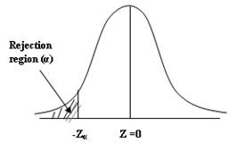
Fig. 16.1 Left tailed Test

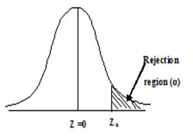
Fig. 16.2 Right tailed Test

16.3.10.2  Two–tailed test

A test of statistical hypothesis where the alternative hypothesis is two–sided such as: H₀: μ=μ₀ against the alternative hypothesis H₁: μ≠μ₀ (μ>μ₀ or μ<μ₀) is known as a two–tailed test and in such a case the critical region is given by the portion of the area lying on both the tails of the probability curve of the test statistic as shown in Fig. 16.3

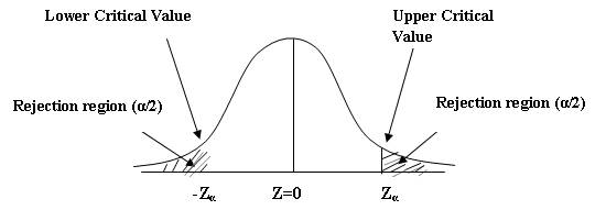
Fig. 16.3 Two Tailed Test

In a particular problem, whether one-tailed or two-tailed test is to be applied depends entirely on the nature of the alternative hypothesis.

16.3.11  Critical values or significant values

The value of a test statistic which separates the critical (or rejection) region and the acceptance region is called the critical value or significant value. It depends upon

· the level of significance and

· the alternative hypothesis, whether it is two tailed or single tailed.

The critical value of the test statistic at α level of significance for a two tailed test is given by Z_α where Z_α is determined by the equation P(|Z| > Z_α), where Z_α is the value so that the total area of the critical region on both tails is α. Since normal probability curve is symmetric curve, we get P[Z>Z_α] = α/2 i.e., the area of each tail is α/2. Thus Z_α is the value such that area to the right of Z_α is α/2 and to the left of - Z_α is α/2 as shown in fig. 16.3 .In case of single tail alternative, the critical value of Z_α is determined so that total area to the right of it (for right tailed test) is α (as shown in fig. 16.2) and for left tailed test the total area to the left of - Z_α is α (as shown in Fig. 16.1).Thus the significant or critical value of Z for a single tailed test (left or right) at level of significance ‘α’ is same as the critical value of Z for a two tailed test at level of significance 2α.

Table 16.2 Critical values of (Z_𝛂) of Z

Critical values (Zα)	Level of significance
	1%	5%	10%
Two tailed test Right tailed test Left tailed test	Zα = 2.33 Zα = -2.33	Zα = 1.645 Zα = -1.645	Zα = 1.28 Zα = -1.28

16.4  Test of Significance

The tests of significance which are dealt hereafter pertain to parametric tests. A statistical test is defined as a procedure governed by certain rules, which leads to take a decision about the hypothesis for its acceptance or rejection on the basis of sample observations. Test of significance enables us to decide on the basis of sample results if

(i) deviation between observed sample statistic and the hypothetical parameter value or

 (ii) the deviation between two sample statistics is significant.

Test of significance is a procedure of either accepting or rejecting a Null hypothesis. The tests are usually called tests of significance since here we test whether the difference between the sample values and the population values or between the values given by two samples are so large that they signify evidence against the hypothesis or these differences are small enough to be accounted for as due to fluctuations of sampling, i.e. they may be regarded as due only to the fact that we are dealing with a sample and not with the whole population. Statistical tests play an important role in biological sciences, dairy industry, social sciences and agricultural sciences etc. The use of these tests is made clear through a number of practical examples:

1. An automatic machine is filling 500 ml. of milk in the pouch. Now to make sure whether the claim is correct or not one has to take a random sample of the filled in pouches and note the actual quantity of milk in the pouches. From these sample observations it would be decided whether the automatic machine is filling the right quantity of milk in the pouches. This is done by performing test of significance.

2. There is a process A which produced certain items. It is considered that a new process B is better than process A. Both the processes are put under operation and then items produced by them are sampled and observations are taken on them. A statistical based test on sample observations will help the investigator to decide whether the process B is better than A or not.

3. Psychologists are often interested in knowing whether the level of IQ of a group of students is up to a certain standard or not. In this case some students are selected and an intelligence test is conducted. The scores obtained by them are subjected to certain statistical test and a decision is made whether their IQ is up to the standard or not.

There is no end to such types of practical problems where statistical tests can be applied. Here one important point may be noted. Whatever conclusions are drawn about the population (s), they are always subjected to some error.

16.5 Steps of Test of Significance

Various steps in test of significance are as follows:

(i) Set up the Null hypothesis H_o.

(ii) Set up the alternative hypothesis H₁ .This will decide whether to go for single tailed test or two tailed test.

(iii) Choose the appropriate level of significance depending upon the reliability of the estimates and permissible risk. This is to be decided before sample is drawn.

(iv) Compute the test statistic .

(v) Compare the computed value of Z in previous step with the significant value Z_α at a given level of significance.

(vi) Conclusion :

a) If |Z| < Z_α i.e. if calculated value of Z (test statistic) is less than Z_α, we say it is not significant, null hypothesis is accepted at level of significance α.

b) If |Z| > Z_α i.e. if calculated value of Z (test statistic) is greater than Z_α , we say it is significant and null hypothesis is rejected at level of significance α.