Module 5. Test of significance

Lesson 19

CHI-SQUARE TEST AND ITS APPLICATIONS

19.1 Introduction

In the preceding lesson some tests of significance were discussed which is based on the assumption that the samples were drawn from normally distributed population. These tests are known as parametric tests as the testing procedure involves the assumption about the type of population of parameters. There are, however, many situations where it is not possible to assume a particular type of population distribution from which the samples are drawn. This leads to development of alternative techniques known as non-parametric or distribution –free methods. Chi-square (χ²) (pronounced as Ki-square) test is one of the important non-parametric test and one of the most commonly used test of significance. The chi-square test dates back to 1900, when Prof. Karl Pearson used it for frequency data classified into k-mutually exclusive categories. It is also a frequently used test in genetics, where one tests whether the observed frequencies in different crosses agree with the expected frequencies or not. The chi-square test is applicable to test the hypothesis of the variance of a normal population, goodness of fit of the theoretical distribution to the observed frequency distribution, in a one way classification having k-categories. It is also applied for the test of independence of attributes, when the frequencies are presented in a two-way classification called the contingency table. In this lesson we give chi-square test of various hypotheses.

19.2 Chi-Square Distribution

If X is a normal variate with mean µ and standard deviation σ viz., X ~ N (μ, σ²) then is a standard normal variate .The square of a standard normal variate i.e., is known as Chi-square (χ²) variate with one degree of freedom (d.f.). If X₁,X₂,---,X_n are n independent random variate following normal distribution with means μ₁,μ₂,---,μ_n and standard deviations σ₁,σ₂,---, σ_n respectively then the variate

which is sum of the squares of n independent standard normal variates , follows Chi-square distribution with n d.f.

19.3  Applications of the χ²−distribution

Chi-square distribution has a number of applications which are enumerated below:

a) To test if the population has a specified value of the variance σ².

b) Chi-square test of goodness of fit.

c) Chi-square test for independence of attributes.

19.3.1  Chi-Square Test for Population Variance:

Suppose on the basis of previous knowledge, we have a preconceived value of population variance σ₀².Suppose we draw a random sample of size n from this population. On the basis of n sample observations (X₁, X₂,…,X_n), the population variance value σ₀² of the population variance σ² is to either be substantiated or refuted with the help of a statistical test. In this case we use Chi-square test. For this the null hypothesis is taken as

and is tested by the statistic

Follows a χ² distribution with (n-1) degree of freedom. Where

is the variance of the sample? If calculated value of chi-square is more than or equal to tabulated chi-square value at α% level of significance then H₀ is rejected at α level of significance otherwise if calculated χ² is less than tabulated χ² at α level of significance then H₀ is not rejected at α level of significance.

Example 1: An owner of a big firm agrees to purchase the product of a factory, if the produced items do not have variance of more than 0.5mm² in their length. To make sure of the specifications, the buyer selects a sample of 18 items from his lot. The length of each item was measured in mm which is given as under:

18.57	18.10	18.61	18.32	18.33	18.46	18.37	18.64	18.58
18.12	18.34	18.57	18.22	18.63	18.43	18.34	18.43	18.63

Test whether the sample has been drawn from the population having specified variance not more than value of 0.5

Solution : On the basis of the sample data, the hypothesis

can be tested by the statistic

 Calculate,   

 For the given data,  

.

Thus,  χ² = 0.515/0.5 = 1.03. Tabulated value of χ² at 5% level of significance and 17 d.f. viz., χ²_0.0517 is 27.587. Since the calculated value of χ² (1.03) is less  than 27.857, we don’t reject  the null hypothesis at α = 0.05. i.e., σ² = 0.5 , It means that the buyer should purchase the lot having specified variance not more than value of 0.5 mm² length .

19.3.2  Chi- square test of goodness of fit

A very powerful test for testing the significance of the discrepancy between theory and experiment was given by Prof. Karl Pearson in 1900 and is known as “chi-square test of goodness of fit”. This test is used for testing the significance of discrepancy between experimental values and the theoretical values obtained under some theory or hypothesis.  It enables us to find if the deviation of the experiment from theory is just by chance or is it really due to the inadequacy of the theory to fit the observed data.

Under the null hypothesis that there is no significant difference between the observed (experimental) values and the theoretical values i.e., there is good compatibility between theory and experiment , Karl Pearson proved that the statistic

Follows a χ² - distribution with (n-1) degree of freedom where O_i (i=1,2,…….,n) is a set of observed (experimental) frequencies and E_i (i=1,2,……..,n) be the corresponding set of expected (theoretical) frequencies obtained under some theory or hypothesis .

If calculated value of χ² is less than the corresponding tabulated value at (n-1) d.f.  then it is said to be non-significant at the required level of significance. This implies that the discrepancy between experimental (observed) values and the theoretical (expected) values obtained under some theory or hypothesis may be attributed to chance. In other words, data do not provide us any evidence against the null hypothesis and we may conclude that there is good correspondence (fit) between theory and experiment. On the other hand if calculated value of χ² is greater than the corresponding tabulated value at (n-1) d.f.  then it is said to be significant at the required level of significance. This implies that the discrepancy between experimental (observed) values and the theoretical (expected) values obtained under some theory or hypothesis cannot be attributed to chance and we reject the null hypothesis. In other words we conclude that the experiment does not support the theory.

Remarks:

 a) The observed and expected frequencies are subjected to a linear constraint where N is the total frequency since it does not involve squares and higher powers of the frequencies. i.e. the sum of deviations of the observed and expected frequencies is always zero.

b) Sometimes the following formula is useful for computation of χ²

where N is the total frequency.

c)  χ²-test depends only on the observed and expected frequencies and on degree of freedom (n-1) .It does not make any assumption regarding the parent population from which the observations care taken .Since χ² does not involve any population parameter it is known as statistic and the test is known as Non-parametric test or Distribution Free test.

19.3.2.1  Degrees of freedom

The number of independent variates which makes up the statistic (e.g., χ²) is known as the degrees of freedom (d.f.). The no. of degrees of freedom in general is the total no. of observations minus the no. of independent linear constraints imposed on the observations. e.g., if k is the no. of independent constraints imposed   on a set of data of n observations then d.f. = (n−k).Thus in a set of n observations usually, the degrees of freedom for χ² are (n – 1), one d.f. being lost because of the linear constraint. . If ‘r’ independent linear constraints are imposed on the cell frequencies, then the d.f. are reduced by ‘r’.

In addition if any of the population parameters (s) is (are) calculated from the given data and used for computing the expected frequencies then in applying χ² test of goodness of fit, we have to subtract one d.f. for each parameter estimated.

19.3.2.2  Conditions for the validity  of χ² test

Following are the conditions which should be satisfied before χ² test can be applied.

(i) N the total number of frequencies must be large, greater than50.

(ii) The sample observations should be independent.

(iii) No theoretical cell frequency should be small. Five should be regarded as the very minimum and 10 is better. The chi-square distribution is essentially a continuous distribution but it cannot maintain its character of continuity if the cell frequency is less than 5). If any theoretical cell frequency is less than 5, then for the application of χ² test, it is pooled with the preceding or succeeding frequency so that the pooled frequency is more than 5 and finally adjusts for the d.f. lost in the pooling.

(iv) The constraints on the cell frequencies, if any, should be linear. Constraints which involve linear especially in the cell frequencies are called linear constraints such as .

The above procedure is explained through following examples:

Example 2 : The following table gives the number of coli forms per ml in thousand bottles of sterilized milk:

No of coli forms (Xi)	0	1	2	3	4	5	6	7	8	9	10
No. of bottles   (fi)	2	8	46	116	211	243	208	119	40	7	0

Fit a binomial distribution to the above data and test the goodness of fit.

Solution

The fitting of this problem is already explained in example 10.6 of lesson 10 (module 3) .In the usual notations we have: n=10, N=1000,

putting r=0,1,2,3,---,10 in f(r) = N x ⁿC_r P^r q^n-r we get the expected frequency as given in the following table:

 Table 19.1

No. of coliforms	No. of bottles (fi) (Oi)		Expected Frequency E i		(Oi - Ei)	(Oi - Ei)^2
0	2	10*	1	11*	-1	1	0.0909
1	8		10
2	46		46		0	0	0.0000
3	116		120		-4	16	0.1333
4	211		207		4	16	0.0773
5	243		246		-3	9	0.0366
6	208		203		5	25	0.1232
7	119		115		4	16	0.1391
8	40		42		-2	4	0.0952
9	7	7*	9	10*	-3	9	0.9000
10	0		1
Total	1000		1000				1.5956

* In the above table since some of  expected cell frequencies being  less than 5 , therefore, they have been merged with either preceding or succeeding frequencies. Accordingly the corresponding observed frequencies have also been merged. Thereafter the value of χ² is calculated as follows

Required Degrees of freedom : 11-1-1-2=7 (n=11,one d.f. is lost due to linear constraint ; one d.f. is lost because the parameter p of binomial distribution is estimated from the given data;2 d.f. are lost due to pooling first and last two frequencies). Tabulated value of χ² for 7 d.f. and at 5% level of significance is 14.067.Since calculated value of χ² is less than tabulated value it is not significant. Thus we conclude that Binomial distribution is a good fit to the given data or Binomial distribution fits well to the given data.

Example 3: The following table gives the number of lactations completed by 1000 cows of Tharparker breed:

No of lactations (Xi)	0	1	2	3	4	5	6	7	8	9	10
No. of females (fi)	300	205	155	126	90	47	35	18	13	8	3

Fit a Poisson distribution to the above data and test its goodness of fit.

Solution :

The fitting of this problem is already explained in example 11.6 of lesson 11 (module 3) . In the usual notations we have :  N=1000,

putting r=0,1,2,3,---,10 in

we get the expected frequency as given in the following table

Table 19.2

No. of lactation (Xi)	No. of Females  (fi)  (Oi)		Expected Frequency (E i)		(Oi - Ei)	(Oi - Ei)^2
0	300		131		169	28447.71	216.6034
1	205		267		-62	3795.93	14.2377
2	155		271		-116	13365.74	49.3911
3	126		183		-57	3261.89	17.81356
4	90		93		-3	8.58	0.092368
5	47		38		9	85.94	2.277851
6	35	77*	13	18*	59	3481.00	193.3889
7	18		4
8	13		1
9	8		0
10	3		0
Total	1000		1000				493.8049

*  In the above table since some of  expected cell frequencies being  less than 5, therefore, they have been merged with either preceding or succeeding frequencies. Accordingly the corresponding observed frequencies have also been merged, Thereafter the value of χ² is calculated as follows

Required Degrees of freedom: 11-1-1-4=5 (n=11,one d.f. is lost due to linear constraint ;one d.f. is lost because the parameter m of Poisson  distribution is estimated from the given data; 4 d.f. are lost due to pooling last five frequencies). Tabulated value of χ² for 5 d.f. and at 5% level of significance is 11. 07. Since calculated value of χ² is more than tabulated value it is significant. Thus, we conclude that Poisson distribution is not a good fit to the given data or Poisson distribution does not fit well to the given data.

19.3.3  Independence of attributes

Let us consider two attributes A and B, A divided into r classes A₁,A₂,………..,A_r and B divided into s classes B₁,B₂,…….B_s. (Such a classification in which attributes are divided into more than two classes is known as manifold classification). The various cell frequencies can be expressed in table known as r×s (manifold) contingency table where (A_i) is the number of persons possessing the attributes A_i (i=1,2,……,r), (B_j) is the number of persons possessing the attributes B_j, (j=1,2,…….,s) and (A_i B_j) is the number of persons possessing both the attributes A_i and B_j, (i=1,2,………,r; j=1,2,……,s). Also  

The problem is to test if two attributes A and B under consideration are independent or not. Under the null hypothesis that the attributes are independent, the theoretical cell frequencies are calculated as

Hence expected frequency for any of the cell frequencies can be obtained by multiplying the row totals and column totals in which the frequency occurs and then dividing the product by the total frequency N.

Table 19.3 rxs Manifold Contingency Table

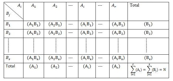
Now for rxs observed frequencies (A_i B_j) and the corresponding expected frequencies E(A_i B_j) . Applying χ² test of goodness of fit, the chi-square statistic is given by

Follows χ² distribution  with (r – 1) (s – 1) d.f. Comparing this calculated value with the tabulated value for (r-1)(s-1) d.f. and at certain level of significance , we reject or accept the null hypothesis of independence of attributes at that level of significance.

19.3.3.1  Degrees of Freedom for rxs contingency table

In (r×s) contingency table in calculation of the expected frequencies, the row totals, the column totals and the grand total remain fixed. Further . Further since the total number of cell frequencies is (r×s), the required number of degrees of freedom is d.f. = rs – (r + s –1) =(r–1) (s–1)

19.3.3.2 2×2 contingency table

Under the null hypothesis of independence of attributes, the value of χ² for the 2x2 contingency table 

			Total
	a	b	a+b
	c	d	c+d
Total	a+c	b+d	N=a+b+c+d

is given by

which follows Chi-square distribution with (2-1)(2-1)= 1 degree of freedom .

19.3.3.3  Yate’s correction for continuity for 2×2 contingency table

In 2×2 contingency table, the no. of d.f. is (2−1) (2−1) =1. If any one of theoretical cell frequency is less than 5, then the using of pooling method for χ² results in χ² with 0 d.f. (since 1 d.f. is lost in pooling) which is meaningless. In this case we apply “Yate’s correction for continuity” which says that add 1/2 to cell frequency which is less than 5 and then adjust for remaining cell frequencies accordingly. The modified formula for χ² is as follows:

If N is large then Yate’s correction will make a very little difference and this can be applied in 2x2 contingency table only.

19.3.3.4 2x r Contingency table:

Under the hypothesis of independence of attributes, the value of χ² for 2xr contingency table:

	2xr Contingency Table					Total
	a1	a2	a3	----	ar
	b1	b2	b3	----	br
Total	m1	m2	m3	----	mr

can be computed from Brandt and Snedecor formula :

Other form of this formula is

which is χ² distribution with (2-1)(k-1)=k-1 d.f. The above procedure is explained through following examples:

Example 4: A milk producer’s union wishes to test whether the preference pattern of consumers for its product is dependent on income levels. A random sample of 500 individuals gives the following data:

Table 19.4

Income	Product Preferred
	Product A	Product B	Product C	Total
Low	170	30	80	280
Medium	50	25	60	135
High	20	10	55	85
Total	240	65	195	500

Can you conclude that the preference patterns are independent of income levels?

Solution: Let us take the hypothesis that preference patterns are independent of income levels. On the basis of this hypothesis, the expected frequencies corresponding to different rows and columns shall be:

and so on. The expected frequencies would be as follows:

 Table 19.5

134.40	36.40	109.20	280
64.80	17.55	52.65	135
40.80	11.05	33.15	85
240	65.00	195.00	500

Applying χ²-test:

Table 19.6

Oi	Ei	(Oi-Ei)^2	(Oi-Ei)^2/Ei
170 50 20 30 25 10 80 60 55	134.60 64.80 40.80 36.40 17.55 11.05 109.20 52.65 33.15	1267.36 219.04 432.64 40.96 55.50 1.10 852.64 54.02 477.42	9.430 3.380 10.604 1.125 3.162 0.099 7.808 1.026 14.402

Degree of freedom = v =(r - 1) (c - 1) = (3 - 1) (3 - 1) = 4

The tabulated value of χ² for 4 d.f. at 5% level of significance i.e., χ²_0.05,4=9.488

Since the calculated value of χ² is greater than the table value, therefore, we reject the null hypothesis and hence conclude that preference patterns are not independent of income levels.

Example 5: In an experiment of cattle from tuberculosis, the following were obtained:

                                    Affected         Not Affected              Total

Inoculated                   4                      20                                24

Not inoculated            6                      50                                56

Total                            10                    70                                80

Calculate χ² and discuss the effect of vaccine in controlling susceptibility to tuberculosis.

Solution : N=80

H_o: The vaccine is not effective in controlling susceptibility to tuberculosis.

H₁: The vaccine is effective in controlling susceptibility to tuberculosis.

Since one of the observed frequency is less than 5. Applying Yate’s correction, we increase the value of that observed frequency by 0.5 and adjust other frequencies. The adjusted observed frequencies after Yate’s correction will be as follows:

	Affected	Not Affected	Total
Inoculated	4+0.5=4.5	20-0.5=19.5	24
Not inoculated	6-0.5=5.5	50+0.5=50.5	56
Total	10	70	80

The tabulated value of χ² for 1 d.f. at 5% level of significance i.e., χ²_0.051 = 3.84. Since the calculated value of χ² is less than the tabulated value, we accept the null hypothesis and hence conclude that the vaccine is not effective in controlling susceptibility to tuberculosis.

Example 6: A milk product factory is bringing out a new product. In order to map out its advertising campaign, it wants to determine whether product appeals equally to all age groups. The following table gives the number of persons who liked or disliked the product in different age groups.

Table 19.7 No. of persons

Preference	Age group (in years)				Total
	< 20	20-30	30-40	> 40
Liked	75	70	60	55	260
Disliked	25	30	40	45	140

Can it be reasonably concluded that the new product appeals equally to all age groups?

Solution:

N = 400

H₀: The new product appeals equally to all age groups.

H₁: The new product does not equally appeal to all the age groups.

Table 19.8

Preference	Age group (in years)				Total
	< 20	20-30	30-40	> 40
Liked	a1=75	a2=70	a3=60	a4=55	n1=260
Disliked	b1=25	b2=30	b3=40	b4=45	n2=140
	m1=100	m2=100	m3=100	m4=100	N=400

=   4.3956(2.5)=10.989

The tabulated value of χ² for 3 d.f. at 5% level of significance i.e., χ²_0.053 = 7.815. Since the calculated value of χ² is greater than the tabulated value, we reject the null hypothesis and hence conclude that the new product did not equally appeal to all the age groups.