Module 7. Correlation and regression

Lesson 23

LINEAR CORRELATION

23.1  Introduction

In the first module we have confined our discussion to univariate distributions only i.e., the distributions involving only one variate and also saw how the various measures of central tendency, dispersion, skewness and kurtosis can be used for the purposes of comparison and analysis. We may, however, come across certain series where each item of the series may assume the values of two or more variables. Such distribution, in which each unit of the series assumes two values, is called a bivariate distribution. Further, if we measure more than two variables on each unit of a distribution, it is called a multivariate distribution. In a series, the units on which different measurements are taken may be of almost any nature such as different individuals, times, places etc.

In our day –to –day life, we find many situations when a mutual relationship exists between two variables i.e., with change (fall or rise) in the value of one variable there may be change (fall or rise) in the value of other variable. At times, an increase in one variable is accompanied by increase or decrease in the other variable. Such changes in variables suggest that there is certain relationship between them.  For example, as price of a commodity increases the demand for the commodity decreases. In milk , the content of total solid decreases with decrease in fat level. Similarly with the increase in the levels of pressure, the volume of a gas decreases at a constant temperature. These facts indicate that there is certainly some mutual relationships that exist between the demand of a commodity and its price, total solid level and fat level and pressure and volume. Such association is studied in correlation analysis. The correlation is a statistical tool which measures the degree or intensity or extent of relationship between two variables and correlation analysis involves various methods and techniques used for studying and measuring the extent of the relationship between the two variables.

23.2  Meaning of Correlation

Correlation is a statistical technique which measures and analyses the degree or extent to which two or more variables fluctuate with reference to one another. It denotes the inter-dependence amongst variables. The degrees are expressed by a coefficient which ranges between -1 to +1. The direction of change is indicated by + or – signs; the former, refers to the movement in the same direction and the later, in the opposite direction. An absence of correlation is indicated by zero. Correlation thus expresses the relationship through a relative measure of change and it has nothing to do with the units in which the variables are expressed.

23.3  Definition of Correlation

Some important definitions are given below:

“If two or more quantities very in sympathy so that movement in the one tend to be accompanied by corresponding movements in the other (s) then they are said to be correlated”.

-L.R. Connor

“Correlation analysis attempts to determine the degree of relationship between variables”.

-Ya-Lun Chou

“When the relationship is of a quantitative nature, the appropriate statistical tool for discovering and measuring the relationship and expressing it in a brief formula is known as correlation.”

-Croxton and Cowden

“Correlation is an analysis of the covariation between two or more variables.”

-A.M. Tuttle

23.4  Types of Correlation

23.4.1  Positive and negative correlation

If the values of the two variables deviate in the same direction i.e., if the increase in the values of one variable results, on an average, in a corresponding increase in the values of the other variable or if a decrease in the values of one variable results, on an average, in a corresponding decrease in the values of the other variable, correlation is said to be positive or direct e.g., relationship between Total solids and SNF in milk, height and weight of student in the class, income and expenditure, demand and production, time and microbial growth in curd.

On the other hand, correlation is said to be negative or inverse if the variable deviate in the opposite direction i.e., if the increase (decrease) in the values of one variable results, on the average, in a corresponding decrease (increase) in the values of the other variable e.g. relationship between fat and SNF in milk, price and demand of a commodity, pressure and volume of a gas, Temperature and microbe number in milk, pH and acidity in milk.

23.4.2  Linear and non–linear correlation

The correlation between two variables is said to be linear if corresponding to a unit change in one variable, there is a constant change in the other variable over the entire range of the values. In general, two variables x and y are said to be linearly related, if there exists a relationship of the form Y = a + bX between them which is the equation of a straight line with slope ‘b’ and which makes an intercept ‘a’ on the y-axis. Hence, if the values of the two variables are plotted as points in the xy-plane, we shall get a straight line. The relationship between two variables is said to be Non-linear or curvilinear if corresponding to a unit change in one variable, the other variable does not change at a constant rate but at fluctuating rate. In such cases if the data are plotted on the XY-plane we do not get a straight line but a curve. Mathematically speaking, the correlation is said to be non-linear if the slope of the plotted curve is not constant.

23.5  Methods of Studying Correlation

We shall confine our discussion to the methods of ascertaining only linear relationship between two variables (series). The commonly used methods for studying the correlation between two variables are

i. Scatter diagram method.

ii. Karl Pearson’s coefficient of correlation. (Covariance method).

iii. Rank method.

23.5.1  Scatter diagram method

Scatter diagram is one of the simplest ways of diagrammatic representation of a bivariate distribution and provides us one of the simplest tools of ascertaining the correlation between two variables. Suppose we are given n pairs of values (X₁, Y₁), (X₂, Y₂),…, (X_n, Y_n) of two variables X and Y. For example if the variables X and Y denote the fat and SNF contents in milk respectively then the pairs (X₁, Y₁), (X₂, Y₂),…, (X_n, Y_n) may represent the fat and SNF contents (in pairs) of n samples of milk. These n points may be plotted as dots (.) on the X-axis and Y-axis in the XY-plane. (It is customary to take the dependent variable along the Y –axis and independent variable along the X-axis.) The diagram of dots so obtained is known as scatter diagram. From scatter diagram we can fairly obtain good, though rough, idea about the relationship between the two variables. The following points may be borne in mind in interpreting the scatter diagram (as shown in Fig. 23.1) regarding the correlation between the two variables:

a) If the points are very dense then a fairly good amount of correlation is expected. On the other hand if the points are scattered than it indicates poor correlation.

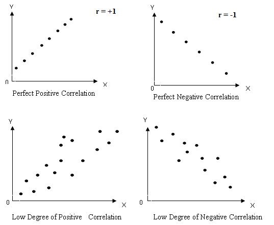
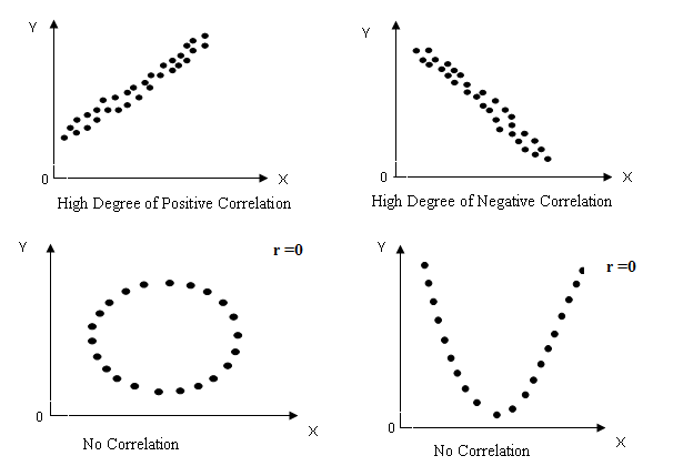
Fig. 23.1 Scatter diagram depicting different forms of correlation

b) If the point on the scatter diagram reveals any trend (either upward or downward) the variables are said to be correlated and if no trend is revealed then variables are uncorrelated.

c) If there is an upward trend rising from lower left hand corner and going upward to the upper right hand corner then correlation is said to be positive. On the other hand the points depict a downward trend from upper left hand corner than correlation is said to be negative.

d) If all the points lie on the straight line starting from the left bottom and going up to right top. The correlation is perfect and positive.

e)   On the other hand if all the points lie on a straight line starting from left top and coming down to right bottom, correlation is perfect and negative.

The major limitation of this method is that it only tells whether there exists a correlation between the variables and its direction. It does not give idea about the precise degree of relationship between the two variables.

23.5.2  Karl pearson’s coefficient of correlation (Covariance method)

A mathematical method for measuring the intensity or the magnitude of linear relationship between two variable series was suggested by Karl Pearson (1867-1936), a great British Bio-metrician and Statistician and is by far the most widely used method in practice.

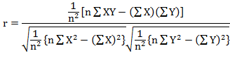
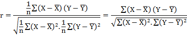
Karl Pearson’s measure, known as Pearsonian correlation coefficient between two variables (series) X and Y, usually denoted by r(X, Y) or r_XY or simply r is a numerical measure of linear relationship between them and is defined as the ratio of the covariance between X and Y, written as Cov (X,Y) to the product of the standard deviations of X and Y. Symbolically,

………(Eq. 23.1)

If (X₁, Y₁), (X₂, Y₂),---, (X_n, Y_n) are n pairs of observations of the variables X and Y in a bivariate distribution, then

………(Eq. 23.2)

summation being taken over n pair of observations. Substituting in (23.1) we get,

………(Eq. 23.3)

Simplifying equation (23.2)          

………(Eq. 23.4)

………(Eq. 23.5)

………(Eq. 23.6)

Similarly we have,

………(Eq. 23.7)

Substituting (23.5), (23.6) and (23.7) in (23.1) we get

………(Eq. 23.8)

The above procedure is illustrated by the following example

Example 1 : The following data pertains to  spoilage of milk (in %)(X) and the temperature (⁰C) (Y) of storage of milk in a dairy plant.

Spoilage of Milk (X)	27.3	29.5	26.8	29.5	30.5	29.7	25.6	25.4	24.6	23.6
Temperature(^0C) (Y)	33.9	34.6	34.5	36.9	37.1	37.3	28.8	29.6	31.2	30.7

Find Karl Pearson’s Correlation Coefficient between spoilage of milk (in %)(X) and the temperature (⁰C) (Y) using different formulae discussed above.

Solution

Calculate means of two variables X and Y and prepare the following table:

Spoilage of Milk (X)	Temperature (^0C) (Y)
27.3	33.9	0.05	0.44	0.0025	0.1936	0.022
29.5	34.6	2.25	1.14	5.0625	1.2996	2.565
26.8	34.5	-0.45	1.04	0.2025	1.0816	-0.468
29.5	36.9	2.25	3.44	5.0625	11.8336	7.7400
30.5	37.1	3.25	3.64	10.5625	13.2496	11.830
29.7	37.3	2.45	3.84	6.0025	14.7456	9.408
25.6	28.8	-1.65	-4.66	2.7225	21.7156	7.689
25.4	29.6	-1.85	-3.86	3.4225	14.8996	7.141
24.6	31.2	-2.65	-2.26	7.0225	5.1076	5.989
23.6	30.7	-3.65	-2.76	13.3225	7.6176	10.074
Total    272.5	334.6			53.3850	91.7440	61.990

Calculate r by using the following formula

prepare the following table

Spoilage of Milk (X)	Temperature (^0C) (Y)
27.3	33.9	745.29	1149.21	925.47
29.5	34.6	870.25	1197.16	1020.70
26.8	34.5	718.24	1190.25	924.60
29.5	36.9	870.25	1361.61	1088.55
30.5	37.1	930.25	1376.41	1131.55
29.7	37.3	882.09	1391.29	1107.81
25.6	28.8	655.36	829.44	737.28
25.4	29.6	645.16	876.16	751.84
24.6	31.2	605.16	973.44	767.52
23.6	30.7	556.96	942.49	724.52
Total  272.5	334.6	7479.01	11287.46	9179.84

Calculate r by using the following formula

23.6  Assumptions of Karl Pearson’s Correlation Coefficient

Karl Pearson’s correlation coefficient is based on the following assumptions:

a) There is linear relationship between the variables X & Y i.e., if the pair observations of both the variables are plotted on a scatter diagram, the plotted points will form a straight line.

b) There is often a cause and effect relationship between the forces affecting the distribution of the observations in the two series. Correlation is meaningless if there is no such relationship.

c) Each of the variables (series) is being affected by a large number of independent contributory causes of such a nature so as to produce a normal distribution. For example, relationships between price and demand, price and supply, total solids and fat contents in milk etc. are affected by several factors such that the series result into a normal distribution.

23.7  Properties of Correlation Coefficient

Correlation coefficient has following properties:

23.7.1  Limits of correlation coefficient

Pearson’s Correlation Coefficient can’t exceed numerically. In other words correlation coefficient lie between -1 to +1 i.e. -1≤r_(X,Y)≤+1

Proof: 

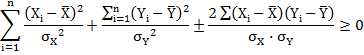
Dividing both sides by n we get;

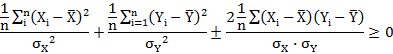
1+1±2r≥0

or,   2(1±r) ≥0

1±r ≥ 0

Either       1+r ≥ 0    i.e. r ≥ −1

      or,      1 – r ≥ 0  i.e. r ≥ +1

Hence r_{(X, Y)} lies between -1 to +1

23.7.2  Correlation coefficient is independent of change of origin and scale

If X_i and Y_i are the given variables and these variables are transformed to new variables U_i and V_i by the change of origin and scale

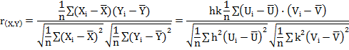
Hence correlation coefficient is independent of change of origin and scale. The procedure is illustrated in the following example by taking the data from example 23.1.

 Example 2 :  Solve example 1 by change of origin and scale:

Solution :  Let us define U_i = X_i – 29.7 and V_i = Y_i – 34.5 prepare the following table

(X)	(Y)
27.3	33.9	-2.4	-0.7	5.76	0.49	1.68
29.5	34.6	-0.2	0	0.04	0	0
26.8	34.5	-2.9	-0.1	8.41	0.01	0.29
29.5	36.9	-0.2	2.3	0.04	5.29	-0.46
30.5	37.1	0.8	2.5	0.64	6.25	2
29.7	37.3	0	2.7	0	7.29	0
25.6	28.8	-4.1	-5.8	16.81	33.64	23.78
25.4	29.6	-4.3	-5	18.49	25	21.5
24.6	31.2	-5.1	-3.4	26.01	11.56	17.34
23.6	30.7	-6.1	-3.9	37.21	15.21	23.79
Total  272.5	334.6	-24.5	-11.4	113.41	104.74	89.92

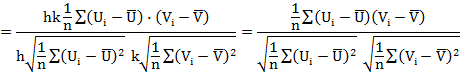
Calculate r by using the following formula

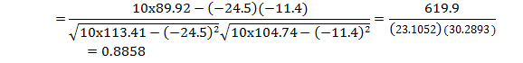
This value is same as obtained in example 1, which shows that correlation coefficient is independent of change of origin.

23.7.3  Two independent variables are uncorrelated but converse is not true

If X & Y are two independent variables then Cov (X, Y) = 0 and hence r = 0 i.e. independent variables are uncorrelated. However, the converse of this result is not true i.e., uncorrelated variables need not necessarily be independent.

23.8  Test of significance of correlation coefficient

As discussed in lesson 18 the correlation coefficient can be tested by t-test. Let a random sample (x_i ,y_i) (i=1,2---,n) of size n has been drawn from a bivariate normal population and let r be the observed sample correlation coefficient . In order to test whether sample correlation coefficient r is statistical significant or there is no correlation between the variables in the population. Prof. R. A. Fisher proved that under the null hypothesis Ho: ρ=0 i.e. the variables are uncorrelated in the population, the statistic

i.e., t follows student’s t distribution with (n-2) d.f. , n being the sample size .

Example 3 Test the significance of sample correlation coefficient obtained in example 1

Solution:  Karl Pearson’s Correlation Coefficient between spoilage of milk (in %)(X) and the temperature (⁰C) (Y) in example 1 was found to be 0.8858 and n=10

 We test the hypothesis Ho: ρ=0 i.e. the variables are uncorrelated in the population vs. H₁: ρ≠0 by the statistic

The tabulated value of t at α=0.05 at 8 d.f. is 2.31.The calculated value of t is more than tabulated value hence it is statistically significant, so we reject H₀.This leads to conclusion that spoilage of milk (in %) and the temperature (⁰C) is highly and significantly correlated.

23.9  Coefficient of Determination

Coefficient of correlation between two variable series measures the linear relationship between them and indicates the amount of variation of one variable which is associated with or is accounted for by another variable. The coefficient of determination, which is given by r², explains to what extent the variation of dependent variable Y is being explained by the explanatory variable X. In other words, the coefficient of determination gives the ratio of the explained variation to the total variation. The coefficient of determination is given by the square of the correlation coefficient i.e. r². Thus,

The quantity (1-r²) is called the coefficient of non-determination or coefficient of alienation. The value of (1-r²) thus measures the deviation from perfect linear relationship. For example if the value of r=0.9, we cannot conclude that 90% of the variation in the relative series (dependent variable) is due to the variation in the subject series (independent variable). But the coefficient of determination in this case is r²=0.81which implies that only 81% of the variation in the relative series has been explained by the subject series and the remaining 19% of the variation is due to other factors.