Module 3. Transportation problem

Lesson 6

INITIAL BASIC FEASIBLE SOLUTION

6.1 Introduction

In the last lesson we have learnt about Transportation Problem (TP) and its formulation. Transportation problem can be solved by simplex method and transportation method. In simplex method the solution is very lengthy and cumbersome process because of the involvement of a large number of decision and artificial variables.  In this lesson we will look for an alternate solution procedure called transportation method in which initial basic feasible solution of a TP can be obtained in a better way by exploiting the special structure of the problem.

6.2 Some Definitions

The following terms are to be defined with reference to Transportation Problem

6.2.1 Feasible solution (FS)

By feasible solution we mean a set of non-negative individual allocations (X_ij ≥ 0) which satisfies the row and column conditions (rim condition).

6.2.2 Basic feasible solution (BFS)

A feasible solution is said to be basic if the number of positive allocations equals m+n-1; that is one less than the number of rows and columns in a transportation problem.

6.2.3 Optimal solution

A feasible solution (not necessarily basic) is said to be optimal if it minimizes the total transportation cost.

6.3 Solution for Transportation Problem

The solution algorithm to a transportation problem can be summarized into following steps:

Step 1: Formulate the problem. The formulation of transportation problem is similar to a LP problem formulation. Here the objective function is to minimize the total transportation cost and the constraints are the supply and demand available at each source and destination, respectively.

Step 2: Obtain an initial basic feasible solution. This initial basic feasible solution can be obtained by using any of the following five methods:

a) North West Corner Rule

b) Minimum cost method

c) Row Minimum Method

d) Column Minimum Method

e) Vogel’s Approximation Method

The solution obtained by any of the above methods must fulfill the following conditions:

i. The solution must be feasible, i.e., it must satisfy all the supply and demand constraints. This is called rim condition.

ii. The number of positive allocations must be equal to m+n–1, where, m is number of rows and n is number of columns.

The solution that satisfies both the above mentioned conditions is called a non-degenerate basic feasible solution.

Step 3: Test the initial solution for optimality. Using any of the following methods one can test the optimality of an initial basic solution:

i. Stepping Stone Method

ii. Modified Distribution Method (MODI)

If the solution is optimal then stop, otherwise, find a new improved solution.

Step 4: Updating the solution. Repeat Step 3 until the optimal solution is obtained.

6.4 Methods of Obtaining an Initial Basic Feasible Solution

Five methods are described to obtain the initial basic feasible solution of the transportation problem. These methods can be explained by considering the following example

Example 1

Let us consider the formulation of TP as given in example 1 of the previous lesson which can be represented by the following e transportation table:

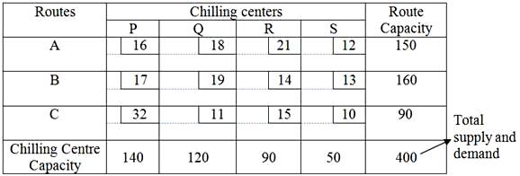
Each cell in the table represents the amount transported from one route to one chilling center. The amount placed in each cell is, therefore, the value of a decision. The smaller box within each cell contains the unit transportation cost for that route.

6.4.1 North west corner rule (NWC) method

Step I: The first assignment is made in the cell occupying the upper left-hand (North West) corner of the transportation table. The maximum feasible amount is allocated there. That is X₁₁ = Min (a₁, b₁) and this value of X₁₁ is then entered in the cell (1, 1) of the transportation table.

Step II: a) If b₁>a₁, we move down vertically to the second row and make the second allocation of magnitude X₂₁=Min. (a₂, b₁- X₁₁) in the cell (2, 1).

b)   If b₁< a₁ we move horizontally to the second column and make the second allocation of magnitude X₁₂ = Min. (a₁–X₁₁, b₂) in the cell (1, 2).

c)   If b₁= a₁, there is a tie for the second allocation. One can make the second allocation of magnitude X₁₂ = Min. (a₁–a₁, b1) = 0 in the cell (1, 2) or X₂₁=Min. (a₂, b₁–b₁) = 0 in the cell (2, 1)

Step III: Repeat steps I & II by moving down towards the lower right corner of the transportation table until all the rim requirements are satisfied.

6.4.1.1 Illustration of north –west corner rule

Let us illustrate the above method with the help of example 1given above. Following North-West corner rule, the first allocation is made in the cell (1,1), the magnitude being X₁₁=Min.(150,140)=140. The second allocation is made in cell (1,2) and the magnitude of allocation is given by X₁₂=Min. (150-140,120)=10. Third allocation is made in the cell (2,2), the magnitude being X₂₂=Min. (160,120-10)=110. The magnitude of fourth allocation in the cell (2,3) is given by X₂₃=Min. (160-110, 90)=50. The fifth allocation is made in the cell (3,3), the magnitude being X₃₃= Min. (90-50, 90)=40. The sixth allocation in the cell (3,4) is given by X₃₄=Min. (90-40, 50) = 50. Now all requirements have been satisfied and hence an initial basic feasible solution to T.P. has been obtained.

 The transportation cost according to the above allocation is given by z = 16 × 140 + 18 × 10 + 19 × 110 + 14 × 50 + 15 × 40 + 10 × 50 = 6310

6.4.2 Matrix minima ( Least cost entry) method

Various steps of Matrix Minima method are given below:

Step I: Determine the smallest cost in the cost matrix of the transportation table. Let it be C_ij. Allocate X_ij = Min. (a_i, b_j) in the cell (i, j).

Step II: a) If X_ij = a_i, cross off the i^th row of the transportation table and decrease b_i by a_i and go to Step III.

              b) If X_ij = b_j, cross off the j^th column of the transportation table and decrease a_i by b_j and go to Step III.

              c) If X_ij = a_i = b_j, cross of either the i^th row or the j^th column but not the both.

Step III: Repeat steps I & II for the resulting reduced transportation table until all the requirements are satisfied. Whenever the minimum cost is not unique, make an arbitrary choice among the minima.

6.4.2.1 Illustration of matrix minima ( Least cost entry) method

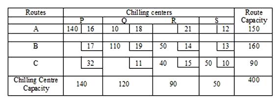
Let us illustrate this method by considering example 1given earlier in this lesson . The first allocation is made in the cell (3, 4) where the cost of transportation is minimum, the magnitude being X₃₄=50. This satisfies the requirement of S chilling centre. Therefore cross off the fourth column. The second allocation is made in the cell (3,2) having minimum cost among remaining cells and its  magnitude being X₃₂=Min.(120,90-50)=40. This satisfies the supply of route C. Cross off the third row. Among the remaining cells, the minimum cost is found in cell (2, 3) so the third allocation is done in cell (2, 3) and its magnitude being X₂₃=Min.(90,160)=90. The requirement of the chilling center R is fulfilled, hence third column is crossed off. Out of the remaining cells the minimum cost is found in cell (1,1) and its magnitude is X₁₁=Min(140,150)=140, as the requirement of chilling center  P is exhausted hence column first is deleted. Among remaining two cells minimum cost is found in cell (1,2) and its magnitude X₁₂=Min(80,150-140)=10 and the last allocation is done in the cell (2,2) and its magnitude is X₂₂=Min(80-10,70)=70. Now all requirements have been satisfied and hence an initial basic feasible solution to T.P. has been obtained and given in the following table.

The transportation cost according to the above allocation is given by z = 16 × 140 + 18 × 10 + 19 × 70 + 11 × 40 + 14 × 90 + 10 × 50 = 5950

6.4.3 Row minima method

Various steps of Row Minima method are given below:

Step I: The smallest cost in the first row of the transportation table is determined, let it be C_ij. Allocate the maximum feasible amount X_ij = Min. (a_i, b_j) in the cell (i, j), so that either the capacity of origin O_i is exhausted or the requirement at destination D_j is satisfied or both.

Step II: a) If X_ij = a₁, so that the availability at origin O₁ is completely exhausted, cross off the first row of the table and move down to the second row.

  b) If X_ij=b_j so that the requirement at destination D_j is satisfied. Cross off the j^th column and reconsider the first row with the remaining availability of origin O₁.

c) If X_ij=a₁=b_j , the origin capacity of O₁ is completely exhausted as well as the requirement at destination D₁ is completely satisfied. An arbitrary choice is made. Cross off the first row and make the second allocation X_1k = 0 in the cell (1, k) with C_1k being the new column cost in the first row. Cross off the first row and move down to the second row.

Step III: Repeat steps I & II for the resulting reduced transportation problem until the requirements are satisfied.

6.4.3.1 Illustration of row minima method

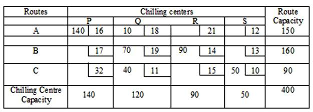
 Let us illustrate this method by considering Example 1given earlier in this lesson. In the first row smallest cost is in the first row which is in the cell (1,4) allocate minimum possible amount X₁₄=Min(50,150)=50. This exhausts requirement of S chilling centre and thus we cross off the fourth column from the transportation table. In the resulting transportation table, the minimum cost in the first row is 16 in the cell (1, 1), the second allocation is made in the cell (1, 1) with X₁₁=Min (140,150-50) =100. This satisfies the supply of Route A, hence first row is deleted. In the second row of the remaining transportation table, the minimum cost is present in cell (2,3) so third allocation is done X₂₃=Min(90,160)=90.This satisfies the requirement of R chilling centre, hence third column is deleted. The next allocation is made in the cell (2,1) with X₂₁=Min(140-100,160-90)=40.This exhausts the requirement of Route P and so we cross-out the first column .The fifth allocation is made in cell X₂₂=Min(120,70-40)=30.This exhausts the supply of route B and hence it is crossed out.  In third row the cell left is (3, 2). Hence the last allocation of amount X₃₂=Min (120-30, 90) =90 is obviously made in the cell (3,2). Now all requirements have been satisfied and hence an initial basic feasible solution of TP has been obtained and given in the following table.

The transportation cost according to the above allocation is given by z = 16 × 100 + 12 × 50 + 17 × 40 + 19 × 30 + 14 × 90 + 11 × 90 = 5700

6.4.4 The column minima method

This method is same as Row minima method except that we apply the concept of minimum cost in column instead of row.

6.4.5 Vogel’s approximation method (VAM)

The Vogel’s Approximate Method takes into account not only the least cost C_ij but also the costs that just exceed C_ij. Various steps of the method are given below:

Step I: For each row of the transportation table identify the smallest and the next to smallest cost. Determine the difference between them for each row. These are called penalties (opportunity cost). Put them along side of the transportation table by enclosing them in parenthesis against the respective rows. Similarly compute these penalties for each column.

Step II: Identify the row or column with the largest penalty among all the rows and columns. If a tie occurs, use any arbitrary tie breaking choice. Let the greatest penalty correspond to i^th row and let c_ij be the smallest cost in the i^th row. Allocate the largest possible amount X_ij = min. (a_i, b_j) in the (i, j) of the cell and cross off the i^th row or j^th column in the usual manner.

Step III: Re-compute the column and row penalty for the reduced transportation table and go to step II. Repeat the procedure until all the requirements are satisfied.

Remarks:

1. A row or column ‘difference’ indicates the minimum unit penalty incurred by failing to make an allocation to the smallest cost cell in that row or column.

2. It will be seen that VAM determines an initial basic feasible solution which is very close to the optimum solution that is the number of iterations required to reach optimum solution is minimum in this case.

6.4.6 Illustration of vogel’s approximation method (VAM)

Let us illustrate this method by considering Example 1 discussed before in this lesson .

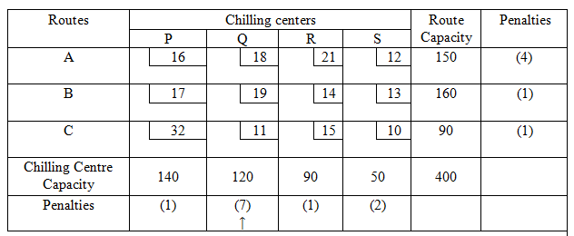
For each row and column of the transportation table determine the penalties and put them along side of the transportation table by enclosing them in parenthesis against the respective rows and beneath the corresponding columns. Select the row or column with the largest penalty i.e. (7) (marked with an arrow) associated with second column and allocate the maximum possible amount to the cell (3,2) with minimum cost and allocate an amount X₃₂=Min(120,90)=90 to it. This exhausts the capacity of route C. Therefore, cross off third row. The first reduced penalty table will be:

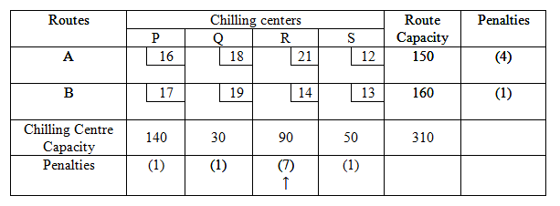
In the first reduced penalty table the maximum penalty of rows and columns occurs in column 3, allocate the maximum possible amount to the cell (2,3) with minimum cost and allocate an amount X₂₃=Min(90,160)=90 to it . This exhausts the capacity of chilling center R .As such cross off third column to get second reduced penalty table as given below.

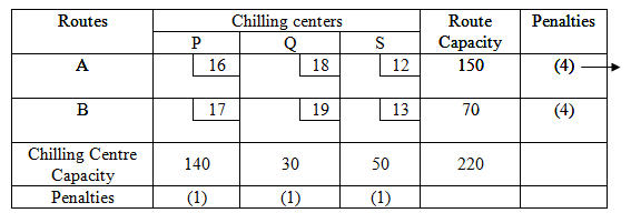
In the second reduced penalty table there is a tie in the maximum penalty between first and second row. Choose the first row and allocate the maximum possible amount to the cell (1,4) with minimum cost and allocate an amount X₁₄=Min(50,150)=50 to it . This exhausts the capacity of chilling center S so cross off fourth column to get third reduced penalty table as given below:

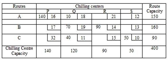
The largest of the penalty in the third reduced penalty table is (2) and is associated with first row and second row. We choose the first row arbitrarily whose min. cost is C₁₁ = 16. The fourth allocation of X₁₁=min. (140, 100) =100 is made in cell (1, 1). Cross off the first row. In the fourth reduced penalty table i.e.  second row, minimum cost occurs in cell (2,1) followed by cell (2,2)  hence allocate X₂₁=40 and X₂₂=30. Hence the whole allocation is as under:

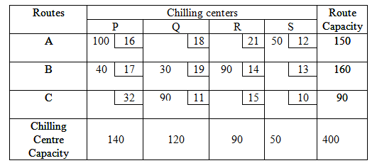
The transportation cost according to the above allocation is given by z = 16 × 100 + 12 × 50 + 17 × 40 + 19 × 30 + 14 × 90 + 11 × 90 = 5700

Note: Generally, Vogel’s Approximation Method is preferred over the other methods because the initial BFS obtained is either optimal or very close to the optimal solution.