Module
3.
Transportation problem
Lesson 7
OPTIMAL SOLUTION
7.1 Introduction
After examining the initial basic feasible solution, the next step is to test the optimality of basic feasible solution. Though the solution obtained by Vogel’s method is not optimal, yet the procedure by which it was obtained often yields close to an optimal solution. So to say, we move from one basic feasible solution to a better basic feasible solution, ultimately yielding the minimum cost of transportation. There are two methods of testing optimality of a basic feasible solution. The first of these is called the Stepping Stone method and the second method is called Modified Distribution method (MODI).By applying either of these methods, if the solution is found to be optimal, then problem is solved. If the solution is not optimal, then a new and better basic feasible solution is obtained. It is done by exchanging a non-basic variable for one basic variable i.e. rearrangement is made by transferring units from an occupied cell to an empty cell that has the largest opportunity cost and then shifting the units from other related cells so that all the rim requirements are satisfied.
7.2 Some Definitions
7.2.1 Non-degenerate solution
A basic feasible solution of an m x n transportation problem is said to be non-degenerate, if it has the following two properties:
(1) Starting BFS must contain exactly (m + n -1) number of individual allocations.
(2) These allocations must be in independent positions.
Here
by independent positions of a set of allocations we mean that it is always
impossible to form closed loops through these allocations. The following table
show the non-independent and independent positions indicated by the following
diagram:

7.2.2 Degeneracy
If the feasible solution of a transportation problem with m origins and n destinations has fewer than m+n-1 positive Xij (occupied cells), the problem is said to be a degenerate transportation problem. Degeneracy can occur at two stages:
a) At the initial stage of Basic Feasible Solution.
b) During the testing of the optimal solution.
To resolve degeneracy, we make use of artificial quantity.
7.2.3 Closed path or loop
This is a sequence of cells in the transportation tableau such that
a) each pair of consecutive cells lie in either the same row or the same column.
b) no three consecutive cells lie in the same row or column.
c) the first and last cells of a sequence lie in the same row or column.
d) no cell appears more than once in the sequence.
7.3 Stepping Stone Method
In this method, the net cost change can be obtained by introducing any of the non-basic variables (unoccupied cells) into the solution. For each such cell find out as to what effect on the total cost would be if one unit is assigned to this cell. The criterion for making a re-allocation is simply to know the desired effect upon various costs. The net cost change is determined by listing the unit costs associated with each cell and then summing over the path to find the net effect. Signs are alternate from positive (+) to negative (-) depending upon whether shipments are being added or subtracted at a given point. A negative sign on the net cost change indicates that a cost reduction can be made by making the change while a positive sign will indicate a cost increase. The stepping stone method for testing the optimality can be summarized in the following steps:
Steps
1. Determine an initial basic feasible solution.
2. Make sure that the number of occupied cells is exactly equal to m+n-1, where m is number of rows and n is number of columns.
3. Evaluate the cost–effectiveness of transporting goods through the transportation routes not currently in solution. The testing of each unoccupied cell is conducted by following four steps given as under:
a. Select an unoccupied cell, where transportation should be made. Beginning with this cell, trace a closed path using the most direct route through at least three occupied cells and moving with only horizontal and vertical moves. Further, since only the cells at the turning points are considered to be on the closed path, both unoccupied and occupied boxes may be skipped over. The cells at the turning points are called Stepping Stone on the path.
b. Assign plus (+) and minus (-) sign alternatively on each corner cell of the closed path traced starting a plus sign at the unoccupied cell to be evaluated.
c. Compute the net change in the cost along the closed path by adding together the unit cost figures found in each cell containing a plus sign and then subtracting the unit cost in each square containing the minus sign.
d. Repeat sub step (a) through sub step (b) until net change in cost has been calculated for all unoccupied cells of the transportation table.
4. Check the sign in each of the net changes .If all net changes computed are greater than or equal to zero, an optimal solution has been reached. If not, it is possible to improve the current solution and decrease total transportation cost.
5. Select the unoccupied cell having the highest negative net cost change and determine the maximum number of units that can be assigned to a cell marked with a minus sign on the closed path, corresponding to this cell. Add this number to the unoccupied cell and to other cells on the path marked with a plus sign. Subtract the number from cells on the closed path marked with a minus sign.
6. Go to step 2 and repeat the procedure until we get an optimal solution.
To demonstrate the application of this method let us take example 1 discussed in lesson 6 for consideration.
Example 1 Find optimal solution of the problem given in example 1 of lesson 6 by stepping stone method.
Solution
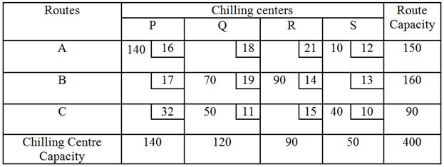
The initial basic feasible solution using Least Cost Method was found in example 1 of previous lesson with the following allocations.
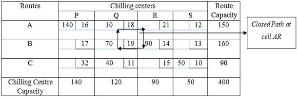
The Transportation cost according to the above allocation is given by
![]()
Beginning at first unoccupied cell (A,Q) trace a closed path and this closed path is AR ⟶ BR ⟶ BQ ⟶ AQ. Assign plus (+) and minus (-) sign alternatively on each corner cell of the closed path traced starting a plus sign at the unoccupied cell .Evaluate the cost–effectiveness of transporting milk on different transportation routes of each unoccupied cell and given in the following table:
|
Unoccupied cell |
Closed Path |
Net Cost change (in Rs.) |
|
(A,R) |
|
21-14+19-18= 8 |
|
(A,S) |
|
12-10+11-18= -5 |
|
(B,P) |
|
17-16+18-19= 0 |
|
(B,S) |
|
13-10+11-19= -5 |
|
(C,P) |
|
32-16+18-11= 23 |
|
(C,R) |
|
15-11+19-14= 9 |
Select the
unoccupied cell having the highest negative net cost change i.e. cell
(A,S). The maximum number of units that can be transported to a cell
marked with a minus sign on the closed path is 10. Add this number to the
unoccupied cell and to other cells on the path marked with a plus sign.
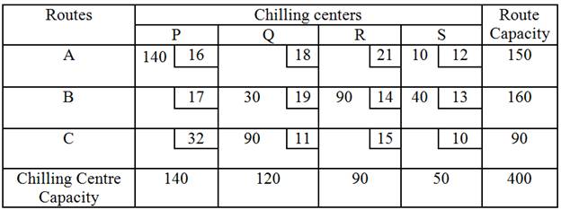
Subtract the number from cells on the closed path marked with a minus sign. New
solution is given in the following table.
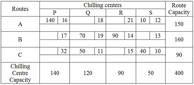
The transportation cost according to the above allocation is given by
![]()
Beginning at the first unoccupied cell (A,Q) and repeating the steps given above. Evaluate the cost–effectiveness of transporting milk on different transportation routes of each unoccupied cell given in the following table:
![]()
|
Unoccupied cell |
Closed Path |
Net Cost change (in Rs.) |
|
(A,Q) |
|
18-12+10-11= 5 |
|
(A,R) |
|
21-12+10-11+19-14= 13 |
|
(B,P) |
|
17-19+11-10+12-16= -5 |
|
(B,S) |
|
13-10+11-19= -5 |
|
(C,P) |
|
32-16+12-10= 18 |
|
(C,R) |
|
15-11+19-14= 9 |
Select the
unoccupied cell having the highest negative net cost change i.e. cell (B,S)
. The maximum number of units that can be transported to a cell marked
with a minus sign on the closed path is 40. Add this number to the unoccupied
cell and to other cells on the path marked with a plus sign. Subtract the
number from cells on the closed path marked with a minus sign. New solution is
given in the following table.
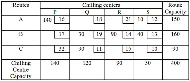
The transportation cost according to the above allocation is given by
![]()
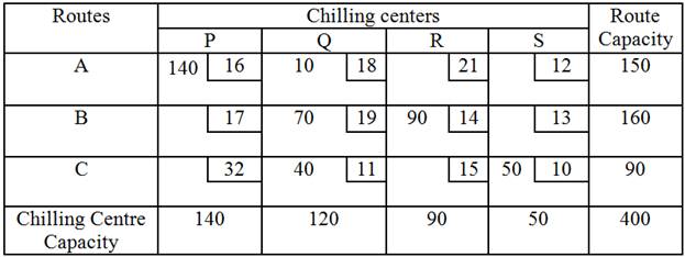
Beginning at the first unoccupied cell (A,Q) and repeating the steps given above. Evaluate the cost–effectiveness of transporting milk on different transportation routes of each unoccupied cell and given in the following table:
|
Unoccupied cell |
Closed Path |
Net Cost change (in Rs.) |
|
(A,Q) |
|
18-12+13-19= 0 |
|
(A,R) |
|
21-12+13-14= 8 |
|
(B,P) |
|
17-16+12-13= 0 |
|
(C,P) |
|
32-16+12-13+14-11= 18 |
|
(C,R) |
|
15-11+19-14= 9 |
|
(C,S) |
|
10-13+19-11= 5 |
Since all the unoccupied cells have positive values for the net cost change, hence optimal solution has reached and optimal cost is Rs. 5700.
7.4 MODI (Modified Distribution) Method
The MODI (Modified Distribution) method is an efficient method of testing the optimality of a transportation solution. In stepping stone method each of the empty cells is evaluated for the opportunity cost by drawing a closed loop. In situations where a large number of sources and destinations are involved, this would be a very time consuming exercise. This method avoids this kind of extensive scanning and reduces the number of steps required in the evaluation of the empty cells. This method allows us to compute improvement indices quickly for each unused square without drawing all of the closed paths. Because of this, it can often provide considerable time savings over other methods for solving transportation problems. It provides new means of finding the unused route with the largest negative improvement index. Once the largest index is identified, we are required to trace only one closed path. This path helps determine the maximum number of units that can be transported via the best unused route. Steps involved for finding out the optimal solution of transportation problem are as follows:
|
1. |
Determine an initial basic feasible solution using any one of the five methods discussed earlier. We start with a basic feasible solution consisting of (m + n – 1) allocations in independent positions. |
|
2. |
Determine a set of (m +n) numbers ur
(r = 1, 2, 3, . . . , m) and vs (s = 1, 2, 3, . . . ,n), such
that, for each occupied cell (r, s) |
|
3. |
Compute
the opportunity cost using
|
|
4. |
Check
the sign of each opportunity cost. If the opportunity costs of all the
unoccupied cells are either positive or zero, the given solution is the
optimum solution. On the other hand, if one or more unoccupied cell has negative
opportunity cost, the given solution is not an optimum solution and further
savings in transportation cost are possible.
|
|
5. |
Select the unoccupied cell with the smallest
negative opportunity cost as the cell to be included in the next solution.
|
|
6. |
Draw a closed path or loop for the unoccupied cell selected in the previous step, using the most direct route through at least three occupied cells and moving with only horizontal and vertical moves. |
|
7. |
Assign alternate plus and minus signs at the unoccupied cells on the corner points of the closed path with a plus sign at the cell being evaluated. |
|
8. |
Determine the maximum number of units that should be transported to this unoccupied cell. The smallest value with a negative position on the closed path indicates the number of units that can be transported to the entering cell. Now, add this quantity to all the cells on the corner points of the closed path marked with plus signs and subtract it from those cells marked with minus signs. In this way an unoccupied cell becomes an occupied cell. |
|
9. |
Repeat the whole procedure until an optimum solution is obtained. |
Let us illustrate this method by taking example 1 into consideration.
Example 2 Find optimal solution of the problem given in example 1 of lesson 6 by MODI method.
Solution
The
initial basic feasible solution using Least Cost Method was found in example 1
of previous lesson with the following allocations.
The transportation cost according
to the above allocation is given by
![]()
Step 1: Since the number of occupied cells are m+n-1=3+4-1=6 the initial solution is non –degenerate. Thus optimal solution can be obtained.
Step 2: We first set up an equation for each occupied cell:
|
|
|
|
|
|
|
|
|
|
|
|
![]()
Step 3: After the row and column numbers have been computed, the next step is to evaluate the opportunity cost for each of the unoccupied cells by using the relationship
![]()
|
Unoccupied cell |
Opportunity Cost |
|
(A,R) |
d13 = 21 – (0+13)= 8 |
|
(A,S) |
d14 = 12- (0+7) = -5 |
|
(B,P) |
d21 = 17 – (1+16) = 0 |
|
(B,S) |
d24 = 13 - (1+17) = -5 |
|
(C,P) |
d31 = 32 – (-7+16) = 23 |
|
(C,R) |
d33 = 15 – (-7+13) = 9 |
Step 4: Select
the unoccupied cell having the highest negative net cost change i.e. cell
(A,S). The maximum number of units that can be transported to
a cell marked with a minus sign on the closed path is 10. Add this number to
the unoccupied cell and to other cells on the path marked with a plus sign.
Subtract the number from cells on the closed path marked with a minus sign. New
solution is given in the following table
The
transportation cost according to the above allocation is given by ![]()
To test this solution for further
improvement, we recalculate the values of ur and vs based on the second solution for each of the
occupied cells.
|
|
|
|
|
|
|
|
|
|
|
|
Again, we again calculate the opportunity costs for each unoccupied cell by using the relationship
![]()
|
Unoccupied cell |
Opportunity Cost |
|
(A,Q) |
d12 = 18-(0+13) = 5 |
|
(A,R) |
d13 = 21-(0+8) = 13 |
|
(B,P) |
d21 = 17 – (6+16) = -5 |
|
(B,S) |
d24 =13 – (6+12) = -5 |
|
(C,P) |
d31 = 32-(-2+16) = 18 |
|
(C,R) |
d33 = 15 – (-2+8) = 9 |
Since the
opportunity cost in the cell (B,P) and (B,S) are negative , the current basic
feasible solution is not optimal and can be improved . Choosing the unoccupied
cell (B,S), we trace a closed path that begins and ends at this cell. The
maximum number of units that can be transported to a cell marked with a
minus sign on the closed path is 40. Add this number to the unoccupied cell and
to other cells on the path marked with a plus sign. Subtract the number from
cells on the closed path marked with a minus sign. New solution is given in the
following table.
To test this solution for further
improvement, we recalculate the values of ur and vs based on the second solution for each of the
occupied cells.
|
|
|
|
|
|
|
|
|
|
|
|
Again, we calculate the opportunity costs for each
unoccupied cell by using the relationship
![]()
|
Unoccupied cell |
Opportunity Cost |
|
(A,Q) |
d12 = 18-(0+18) = 0 |
|
(A,R) |
d13 = 21-(0+13) = 8 |
|
(B,P) |
d21 = 17 – (1+16) = 0 |
|
(C,P) |
d31 = 32-(-7+16) = 23 |
|
(C,R) |
d32 = 15 – (-7+13) = 9 |
|
(C,S) |
d34 = 10 – (-7+12) = 5 |
In the above
table the opportunity costs for each unoccupied cell is positive value, we
conclude that solution is optimal one and the transportation cost is ![]()
7.5 Maximization in a Transportation Problem
Although the transportation problems
which were dealt so far were of minimization, we may also come across of
transportation problems with maximization objectives. When origins are related
to destinations by a profit function instead of cost, the objective is to be
maximize instead of minimize. The most convenient way to deal with the
maximization case is to transform the profits to relative costs which are
carried out by subtracting the profit associated with each cell from the
largest profit in the matrix. Once the optimal solution for the minimization
problem is obtained, the value of objective function is determined with
reference to the original profit matrix.