Module 1. Introduction to computer programming

Lesson 1

PROBLEM SOLVING WITH COMPUTER PROGRAMMING – PART I
(Algorithms and Flowcharts)

1.1  Introduction

A programming language is a systematic notation by which we describe computational processes to others. Computational process in present context means a set of steps that a machine can perform for solving a problem. However, computers, unfortunately, do what we tell them to do, not necessarily what we want them to do! There must be no ambiguity in the instructions that we give to a computer in our programmes, i.e., no possibility of alternative interpretations. Since the computer always takes some course of action, great care must be taken to ensure that there is only one possible course of action so that we get the desired results. For instance, consider the statement: “Compute arithmetic mean for a given set of n observations”. It seems to specify the computation we wish to get performed by computer. However, it is in fact too imprecise for computer to do the desired calculations, because too much detail is left unspecified, e.g., where are the observed values, how many are there, are the missing/zero values to be included, and so on. This is the essence of computer programming. 

Most interesting problems appear to be very complex from programming standpoint. For some problems such as mathematical problems, this complexity may be inherent in the problem itself. In many cases, however, it can be due to other factors that may be within our control, e.g., incomplete or unclear specifications of the problem. In the development of computer programmes, complexity need not always be a problem if it can be properly controlled.

Computer programming can be difficult. However, we can do a great deal to make it easier. First, it is important that we separate the problem-solving phase of the task from implementation phase (Fig.1.1). In the former phase, we concentrate on the design of an algorithm to solve the stated problem. Only after ensuring that the formulated algorithm is appropriate, we translate the algorithm in some programming language such as ‘C’. Given an algorithm that is precise, its translation into a computer programme is quite straightforward.

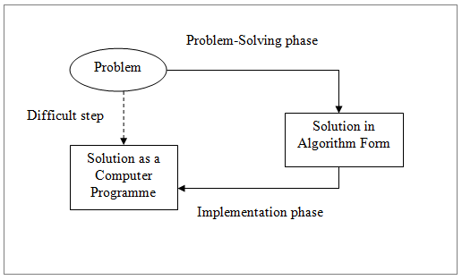
Fig. 1.1 Problem solving with computer

Hence, the essence of computer programming is the encoding of algorithms for subsequent execution on automatic computing machines. The notion of an algorithm is one of the basic ideas in mathematics and has been known and used since initial theories of Computer Science emerged. However, we can define the term algorithm in computer programming context as follows:

An algorithm is a list of instructions specifying a sequence of operations, which will give the answer to any problem of a given type.

There are following six basic operations performed through a computer programme:

1. Input data

a) Read data from a file

b) Get data from the keyboard

2. Perform arithmetic computations using actual mathematical symbols or the words for the symbols

3. Assign a value to a variable

There are three cases possible:

a) Variable initialisation

b) Assign a value to a variable as a result of some processing 

c) Keep a piece of information for later use (Save/Store)

4. Compare two pieces of information and select one of two (or more) alternative actions   

5. Repeat a group of actions on the basis of some pre-defined condition or number of iterations

6. Output information

a) Write information to a file

b) Display information to the screen.

1.2  Properties of an Algorithm

Algorithms have several properties of interest: a) in general, the number of operations, which must be performed in solving a particular problem is not known beforehand; it depends on the particular problem and discovered only during the course of computation; b) the procedure specified by an algorithm is deterministic process, which can be repeated successfully at any time and by anyone; it must be given in the form of a finite list of instructions giving exact operation to be performed at each stage of the calculations; and c) the instructions comprising an algorithm define the task that may be carried out on any appropriate set of initial data and which, in each case, give the correct result. In other words, an algorithm tells how to solve not just one particular problem, but a whole class of similar problems.

1.3 Description of Algorithms

There are several approaches possible to the description of algorithms, viz., narrative description, the flowchart, an algorithmic language, etc.

Narrative approach

It is a straightforward method of expressing an algorithm, i.e., simply to outline its steps verbally. Recipes, for example, are normally expressed in this fashion. This is easy to do. However, natural language is wordy and imprecise and often quite unreliable as a vehicle for transferring information. Hence, natural language is unsuitable as the sole medium for the expression of algorithms. Despite its drawbacks, however, prose (i.e., ordinary language without metrical structure) does have a place, possibly in presenting clarifying remarks or outlining special cases. Hence, it is not discarded entirely.

An illustration: Consider to design an algorithm to compute arithmetic mean for a given set of n observations using narrative approach.

1.      Read the value of n (i.e., number of observations)

2.      Read all then n observations one-by-one

3.     Add these n observations x1, x2, ...

4.      Divide the ‘sum’ obtained in step-3, by n to calculate mean

5.      Write the mean value obtained in step-4

6.      Stop

The flowchart

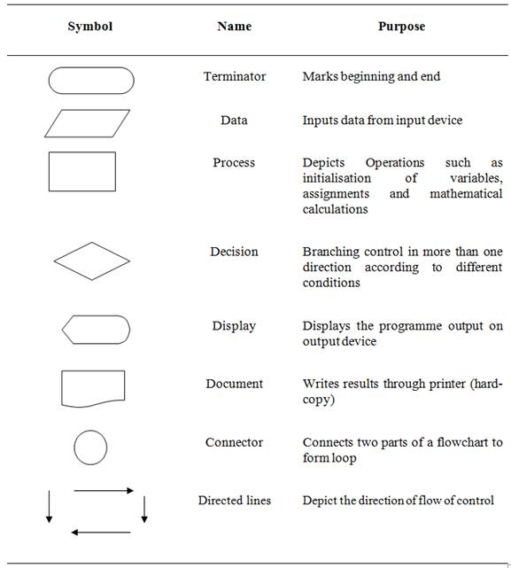
It is often easier to convey ideas pictorially than verbally. Maps provide a convenient representation of the topology of a city, and may be of more value when you are lost than verbal directions. Assembly directions for a newly acquired piece of equipment are usually much more comprehensible if diagrams are included. A very early attempt at providing a pictorial format for the description of algorithms, which dates back to the days of von Neumann, involved the use of the flowchart. A flowchart shows the logic of an algorithm, emphasising the individual steps and their interconnections. Over the years, a relatively standard symbolism has emerged (see Table-1.1); e.g., computations are represented by a rectangular shape, a decision by a diamond shape, etc. The boxes are connected by directed lines indicating the order in which the operations are to be carried out.

Table 1.1 Flowchart symbols and description

A simple flowchart for the above problem is shown in Fig.1.2.

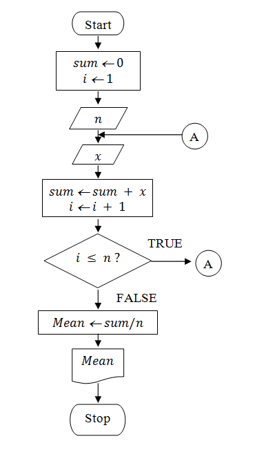
Fig. 1.2 Flowchart to compute average of n observations.

An algorithmic approach

Here, the approach is to extract the best features of the previous two approaches and combine these in a special language for the expression of algorithms. From the narrative approach, we borrow the descriptiveness of prose. To this, we add the conciseness of expression of the flowchart. The result is a kind of ‘pidgin programming language’, similar in flavour to several programming languages. We should try to avoid tying the algorithmic language too closely with any particular programming language.

Example1(a): Simple algorithm to compute average of n observations.

Let us try to design a simple algorithm using the algorithmic approach for the same example to compute average of n observations as follows.

1. [Initialise variables]

sum ← 0

i←1

2. [Input number of observations (n)]
Read (n)

3. [Input n observations (x) one-by-one]
Read (x)

4. [Add the x values one-by-one]
sum ← sum + x
i ← i + 1

5. [Check whether i ≤ n]
if i ≤ n
then go to step-3
else go to step-6

6. [Compute mean value]
mean ← sum/ n

7. [Print the mean value]
Write(‘Mean =’, mean)

8. Exit.

Note that the above algorithm uses goto instructions to perform iteration. Edsger W. Dijkstra, the famous Dutch computer scientist who is well known for his contribution to the fields of algorithm design and programming languages, pointed out in a paper (Dijkstra, 1968) that the goto statement in programming languages should be abolished! This paper was written at a time when the conventional way of programming was to code iterative loops, if ... then ... else  and other control structures by the programmer using goto statements as shown in the preceding algorithm. Most programming languages of that time did not support the basic control flow statements that we take for granted today; or merely provided very limited forms of the same. However, Dijkstra did not mean that all uses of goto were bad, but rather he highlighted the need for superior control structures that, when used properly, would eliminate most of the uses of goto, which was popular at that time. Dijkstra still allowed for the use of goto for more complicated programming control structures. Hence, a new paradigm called structured programming (to be discussed later) was emerged. The sophisticated structured programming languages like ‘C’ discourage the use of goto statements and rather provide proper control and looping structures such as if ... then ... else , while ... do loop, report ... until loop and for loop, which are discussed later (in perspective with ‘C’ programming) in greater details.

Now, let us revise the above algorithm so as to do the same task using a while ... do kind of looping mechanism (also called pre-test loop, as it tests for a condition prior to running a block of code), which executes the underlying set of instructions as long as a pre-defined condition is fulfilled. If the condition is not true at the onset, the loop even does not execute at all in such a case. Mind that while ... do loop is useful when you do not know exactly as to how much iteration the loop has to perform; for instance, in present example, the number of observations may vary for different datasets to be analysed by the programme.

Example 1(b): Revised algorithm to compute average of n numbers using while ... do loop.

1. [Initialise variables]
sum ← 0

i←1

2. [Input number of observations (n)]
Read (n)

3. [set up a while loop, which continues unless  i > n]
while i ≤  n do
          [Input n observations (x) one-by-one]
Read (x)
          [Add the x  values one-by-one]
sum ← sum + x
     i ← i + 1
end while

4. [Compute mean value]
mean ← sum/ n

5. [Print the mean value]
Write(‘Mean =’, mean)

6. Exit.

Further, let us modify the above algorithm so as to perform the same task using a repeat ... until kind of looping structure (also called post-test loop, as it tests the condition after running a block of code once), which executes the underlying set of instructions as long as a pre-defined condition is fulfilled. Even if the condition is not true, the loop executes at least once in such a case. Note repeat ... until  loop is useful like while ... do loop, when you do not know exactly as to how much iteration the loop has to perform; e.g., in present example, the number of observations may vary for different datasets to be analysed by the programme.

Example 1(c): Revised algorithm to compute average of n numbers using repeat ... until  loop.

1 [Initialise variables]
sum ← 0

i←1

2 [Input number of observations (n)]
   Read(n)
3 [set up a repeat…until loop, which continues as long as  i ≤  n is true]
do
          [Input n observations (x ) one-by-one]
Read(x)
          [Add the x  values one-by-one]
sum ← sum + x
i ← i + 1
  while i ≤  n

4 [Compute mean value]
mean ← sum/ n

5 [Print the mean value]
Write(‘Mean =’, mean)

6 Exit.

In case, it is known beforehand as to how much iteration the loop would exactly perform, you can make use of the for loop (also known as count loop). The purpose of for loop is to execute an initialisation, then keep executing a block of statements and updating an expression while a condition is true. It is of the form:

 for (initialization, condition, update)

        Block of statements

end for

This is illustrated with the following example.

Example 1(d): An algorithm to compute average of any ten numbers using for loop.

1. [Initialise variables]
sum ← 0

2. [set up a ‘for’ loop, which iterates ten times]
for i ← 1, i ≤ 10, i ←i + 1 do
          [Input n observations (x) one-by-one]
Read(x)
          [Add the x values one-by-one]
sum ← sum + x
end for

3. [Compute mean value]
mean ← sum/ 10.0

4. [Print the mean value]
Write(‘Mean =’, mean)

5. Exit.

Note that here the variable i is not incremented after each iteration as the for  statement automatically takes care of it. It performs exactly the specified iterations.

Moreover, there is another commonly used control structure called the selection structure. It represents the decision-making capabilities of the computer. This structure facilitates you to make a choice between available options. These choices are based on a decision about whether the respective condition is true or false.

There are many variations of the selection structure as follows:

1. Simple selection (simple if statement): applicable in case a choice is to be made between two alternatives. The keywords used are if,then, else and endif.

2. Simple selection with null false branch (null else statement): This is useful in case a task is performed only when a particular condition is true. The keywords used are if, then and endif..

3. Combined selection (combined if statement): This is used where the statement contains compound conditions. If the conditions are combined using the connector ‘and’, both conditions must be true for the combined condition to be true. If the connector ‘or’ is used to combine any two conditions, only one of the conditions needs to be true for the combined condition to be considered true. The keywords used are if, then and endif. Also, the ‘not’ operator is used for the logical negation of a condition and can be combined with the ‘and’ as well as ‘or’ operators. In order to avoid any ambiguity arising due to several conditions connected through ‘and’ or ‘or’ operators, better use parentheses to make the logic clear.

4. Nested selection (nested if statement): This is useful when the keyword if appears more than once with an if  statement. It uses if, then, else and endif  keywords. Nesting can be classified as linear or non-linear. The linear nested if  statement is used when a field is being tested for various values and a difference action is taken for each value. Each else statement immediately follows its corresponding if condition. A non-linear nested if occurs when a number of different conditions need to be satisfied before a particular action is taken. An else statement can be separated from its corresponding if statement. Avoid using non-linear nested if statements as their logic is often hard to follow. Generally, indention is used for readability. 

Example 2: An algorithm to input an examination’s marks of n students as well as to test each student’s marks for the award of a grade. The marks are assigned as a whole number in the range: 1 to 100. Grades are awarded according to the following criteria:

Serial Number	Criterion	Grade
1.	marks >= 80	Distinction
2.	marks >= 60 but < 80	Merit
3.	marks   >=   40  but   <   60	Pass
4.	marks   <   40	Fail

1. Read (n)

2. i ← 1

3. while i ≤ n do
       Read (marks for one student at a time)
if (marks ≥ 80)
Write(‘Distinction’)
else if (marks ≥ 60 and marks <  80)
Write(‘Merit’)
else if (marks ≥ 40 and marks < 60)
Write(‘Pass’)
else if (marks < 40)
Write(‘Fail’)
end if
i ← i + 1
end while

4. Exit.

Example 3: An algorithm to find and print the largest number among any n given numbers.  

1. Read(n, current_number)

2. max ← current_number

3. counter ← 1

4. while (counter < n) do
counter ← counter +1
Read (next_number)
if (next_number > max) then
max ← next_number
end if
end while

5. Write (‘The largest number is :’, max)

6. Exit.

The above algorithms (Examples 2 and 3) nest if ... then ... endif  structure within the while ... do loop structure. A care should be exercised while creating nested structures. The inner most structure should be properly embedded within the outer structure. Overlapping between the two is not permissible; e.g., in the above algorithm, if structure should not continue after the terminal statement of the while ... do  loop, i.e., while .