Module 1. Descriptive statistics
Lesson 4
MEASURES OF DISPERSION
4.1 Introduction
In the preceding lesson, we have seen different measures of central tendency and learnt how they can be calculated for varying types of distributions. The measures of central tendency are just different types of averages and do not indicate the extent of variability in a distribution. Averages or the measures of central tendency give us an idea of the concentration of the observations about the central part of the distributions. If we are given the average of a series of observations, we cannot form complete idea about the distribution since there may exist a number of distributions whose averages are same but they may differ widely from each other in a number of ways. Let us consider two series I and II of 6 items each
Series Total Mean
I 20 20 25 25 30 30 150 25
II 15 20 25 25 30 35 150 25
We notice that there is no difference as far as the average is concerned. But we notice that in the first case the observations vary from 20 to 30 and in the second case, the observations vary from 15 to 35 i.e. we notice that the greatest deviation from the mean in the first case is 5 and in the second case it is 10. Clearly this indicates a difference in the two series. Such a variation is called scatter or dispersion. Thus, the measures of central tendency must be supported and supplemented by some other measures. One such measure is dispersion. Measures of dispersion help us to study variability of the items i.e. the extent to which the items vary from one another and also from the central value.
4.2 Meaning of Dispersion
The term dispersion is generally used in two senses. Firstly, dispersion refers to the variation of the items among themselves. If the value of all the items of a series is the same, there will be no variation among the various items and the dispersion will be zero. On the other hand, the greater the variation among different items of a series, the more will be the extent of dispersion. Secondly, dispersion refers to the variation of the items about an average. If the difference between the value of items and the average is large, the dispersion will be high and on the other hand if the difference between the values of items and average is small, the dispersion will be low. Thus, dispersion is defined as scatteredness around central value or the spread of the individual items in a given series. According to A. L. Bowley “Dispersion is the measure of the variation of the items”. Spiegel defined dispersion as “The degree to which numerical data tend to spread about an average value is called the variation or dispersion of the data”.
4.3 Objectives of Measuring Dispersion
The measures of dispersion are helpful in statistical investigation. Some of the main objectives of dispersion are:
- To determine the reliability of
an average.
- To compare the variability of
two or more series.
- For facilitating the use of
other statistical measures.
- Basis of Statistical Quality
Control.
4.4 Characteristics for an Ideal Measure of Dispersion
The following are the essential requisites for an ideal measure of dispersion:
· It should be rigidly defined.
· It should be based on all observations.
· It should be readily comprehensive.
· It should be easily calculated.
· It should be amenable to further mathematical treatment.
· It should be affected as little as possible by fluctuations of sampling.
· It should not be affected much by extreme observations.
4.5 Absolute and Relative Measures of Dispersion
The measures of dispersion which are expressed in terms of the original units of a series are termed as Absolute Measures. Such measures are not suitable for comparing the variability of the two distributions which are expressed in different units of measurement. On the other hand, relative measures of dispersion are obtained as ratios or percentages and are thus pure numbers independent of the units of measurement. These measures are used to compare two series expressed in different units.
4.6 Measures of Dispersion
Various measures of dispersion in common use are:
4.6.1 Range
The simplest possible measure of dispersion is the range which is nothing but the difference between the greatest and the smallest observation of the distribution. Thus, Range =Xmax -Xmin where Xmax is the greatest observation and Xmin is the smallest observation of the variable value. In case of the grouped frequency distribution range is defined as the difference between upper limit of the highest class and the lower limit of the smallest class. In order to compare the variability of the two or more distributions given in different units of measurement, the relative measure , called coefficient of range is used and this is defined as follows:
![]()
In other words coefficient of range is the ratio of the difference between two extreme observations of the distribution to their sum.
4.6.1.1 Merits and demerits of range
Range is the simplest though crude measure of dispersion. It is rigidly defined, readily comprehensible and easiest to compute. It got the following drawbacks
- It is not based on all the
observations.
- It is very much affected by
fluctuations of sampling.
- It is unreliable measure of the
dispersion.
- It cannot be used if we are
dealing with open end classes.
- Range is not suitable for
mathematical treatment.
4.6.1.2 Uses of range
In spite of above limitations range as a measure of dispersion, has following applications
- In a number of fields where the
data have small variations like in stock market fluctuations, the
variations in money rates and rate of exchange .
- It is used in industry for the
statistical quality control of the manufactured products by the
construction of R chart i.e. the control chart for range.
- It is also used as a very
convenient measure by meteorological department for weather forecasts.
4.6.2 Quartile deviation or semi-inter-quartile range
The difference between the upper and
lower quartiles i.e. Q3 – Q1 is known as the
inter-quartile range and half of this difference i.e. ![]() (Q3 – Q1) is called the
semi-inter-quartile range or the quartile deviation denoted by Q.D. For
comparative studies of variability of two distributions the relative measure
which is known as Coefficient of Quartile deviation which is given by
(Q3 – Q1) is called the
semi-inter-quartile range or the quartile deviation denoted by Q.D. For
comparative studies of variability of two distributions the relative measure
which is known as Coefficient of Quartile deviation which is given by
![]()
4.6.2.1 Merits of quartile deviation
- The quartile deviation is easy
to compute and understand.
- It is a better measure of
dispersion than range because it makes use of 50% of the data.
- It is not affected at all by
extreme observations.
- It can be computed from the
frequency distribution with open end classes.
4.6.2.2 Demerits of quartile deviation
- It is not based on all the
observations.
- It is affected considerably by
fluctuations of sampling.
- It is not suitable for further
mathematical treatment.
4.6.3 Mean deviation or average deviation
This measure of dispersion is obtained by taking the arithmetic mean of the absolute deviations of the given values from a measure of central tendency. According to Clark and Schkade: “Average deviation is the average amount of scatter of the items in a distribution either the mean or the median, ignoring the signs of deviations. The average that is taken of the scatter is an arithmetic mean, which accounted for the fact that this measure is often called the mean deviation”.
4.6.3.1 Calculation of mean deviation
If X1, X2, ---, Xn are n given observations then mean deviation (M.D.) about an average A is given by:
M.D.
(about an average A) = ![]() Where
Where ![]() read as mod (Xi-A) is the modulus
value or absolute value of the deviation and A is one of the averages viz.,
Mean (M), Median (Md) and Mode (Mo)
read as mod (Xi-A) is the modulus
value or absolute value of the deviation and A is one of the averages viz.,
Mean (M), Median (Md) and Mode (Mo)
In case of grouped frequency distribution, mean deviation about an average A is given by:
M.D.
(about an average A) = ![]() where Xi is the mid value of the
class interval, fi is the corresponding
frequency,
where Xi is the mid value of the
class interval, fi is the corresponding
frequency, ![]() is the total frequency.
is the total frequency.
Mean deviation is minimum when it is calculated from median. In other words, mean deviation calculated about median will be less than the mean deviation about mean or mode. The relative measures of mean deviation is called coefficient of mean deviation is given by
![]()
![]()
![]()
![]()
The coefficients of mean deviations defined above are pure numbers independent of units of measurement and are useful for comparing the variability of different distributions. The calculation of various measures is illustrated in example 1.
Example 1: Find
mean deviation from mean, median and mode using the data given in example 1 of
Lesson 2. Also find the coefficient of mean deviation about mean, median and
mode.
Solution :
Using
the values of Mean (M) =1910 Median (Md) =
1890.8696 and Mode (Mo) = 1866.3636, calculated in Lesson 3and then
prepare the following table:
|
Class Interval |
Mid-value (Xi) |
frequency (fi) |
Xi-M |
|
Xi-Md |
|
Xi-Mo |
|
|
1630-1730 |
1680 |
17 |
-230 |
3910 |
-210.87 |
3584.7832 |
-186.364 |
3168.1812 |
|
1730-1830 |
1780 |
19 |
-130 |
2470 |
-110.87 |
2106.5224 |
-86.3636 |
1640.9084 |
|
1830-1930 |
1880 |
23 |
-30 |
690 |
-10.8696 |
250.0008 |
13.6364 |
313.6372 |
|
1930-2030 |
1980 |
16 |
70 |
1120 |
89.1304 |
1426.0864 |
113.6364 |
1818.1824 |
|
2030-2130 |
2080 |
14 |
170 |
2380 |
189.1304 |
2647.8256 |
213.6364 |
2990.9096 |
|
2130-2230 |
2180 |
7 |
270 |
1890 |
289.1304 |
2023.9128 |
313.6364 |
2195.4548 |
|
2230-2330 |
2280 |
2 |
370 |
740 |
389.1304 |
778.2608 |
413.6364 |
827.2728 |
|
2330-2430 |
2380 |
2 |
470 |
940 |
489.1304 |
978.2608 |
513.6364 |
1027.2728 |
|
Total |
|
100 |
|
14140 |
|
13795.6528 |
|
13981.8192 |
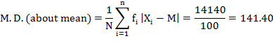
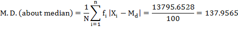
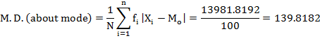
From above calculations we can verify that mean deviation calculated about median (137.9565) is less than mean deviation about mean (141.10) or mode (139.8182).
![]()
![]()
![]()
4.6.3.2 Merits of mean deviation
· It is rigidly defined, easy to understand and calculate.
· It is based on all observations and is better than range and quartile deviation.
· The averaging of the absolute deviations from an average irons out the irregularities in the distribution and thus provides an accurate measure of dispersion.
· It is less affected by extreme observations.
4.6.3.3 Demerits of mean deviation
· Ignoring the signs is not correct from mathematical point of view.
· It is not an accurate method when it is calculated from mode.
· It is not capable of further mathematical treatment.
· It cannot be used if we are dealing with open end classes.
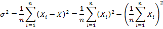
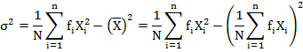
4.6.4 Standard deviation
Standard
deviation, usually denoted by the Greek alphabet σ was first suggested by Karl Pearson as a measure of
dispersion in 1893. It is defined as the positive square root of the mean of
the square of the deviations of the given observations from their arithmetic
mean. If X1,X2,---, Xn is a set of n observations then its standard
deviation is given by :
![]() is the arithmetic
mean.
is the arithmetic
mean.
In case of a grouped data, the standard deviation is given by:
Thus
![]()
Where;
Xi is the value of the variable or
mid value of the class in case of grouped frequency distribution;
fi
is the corresponding frequency of the value Xi,
![]() is the total
frequency
is the total
frequency
![]() is
the arithmetic mean of the distribution.
is
the arithmetic mean of the distribution.
The
square of the standard deviation viz., σ2 is called variance or
second moment about mean.
4.6.4.1 Computation of variance (Direct method)
Other formulae for calculating variance is
and in case of grouped data is
4.6.4.2 Short–cut method (Change of origin)
This method consists in taking deviations of the given observations from any arbitrary value A. The formula for calculation of the arithmetic mean is
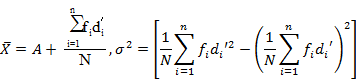
The variance and consequently the standard deviation of a distribution is independent of the change of origin. Thus, if we add (subtract) a constant to (from) each observation of the series, its variance remains same.
4.6.4.3 Step- deviation method (Change of origin and scale)
In case of grouped frequency
distribution, with class intervals of equal magnitude, the calculations are
further simplified by taking; ![]() where Xi is the mid value of the class
and h is the common magnitude of the class intervals. So the formula for
calculating mean and variance is
where Xi is the mid value of the class
and h is the common magnitude of the class intervals. So the formula for
calculating mean and variance is
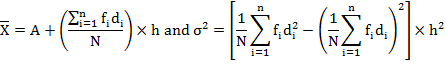
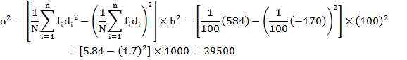
which shows that the variance or standard deviation is not independent of change of scale. Thus, if we multiply (divide) each observation of the series by a constant h, its variance will be multiplied (divided) by h2.Hence variance and consequently the standard deviation of a distribution is independent of the change of origin but not of the scale. The procedure is illustrated in the example 2.It will be seen that the answer in each of the three cases is the same. The step-deviation method is the most convenient on account of simplified calculations.
Example
2: Find variance of the data given in example 1 of Lesson 3 with
short-cut and step-deviation method.![]()
Solution: Prepare the following table to calculate variance by different methods.
|
Class
Interval |
Mid-value
(Xi) |
freq (fi) |
fi
Xi |
fiXi2 |
di’=Xi-A A=2080 |
fi
di’ |
fi
di’2 |
|
fi
di |
fi
di2 |
|
1630-1730 |
1680 |
17 |
28560 |
47980800 |
-400 |
-6800 |
2720000 |
-4 |
-68 |
272 |
|
1730-1830 |
1780 |
19 |
33820 |
60199600 |
-300 |
-5700 |
1710000 |
-3 |
-57 |
171 |
|
1830-1930 |
1880 |
23 |
43240 |
81291200 |
-200 |
-4600 |
920000 |
-2 |
-46 |
92 |
|
1930-2030 |
1980 |
16 |
31680 |
62726400 |
-100 |
-1600 |
160000 |
-1 |
-16 |
16 |
|
2030-2130 |
2080 |
14 |
29120 |
60569600 |
0 |
0 |
0 |
0 |
0 |
0 |
|
2130-2230 |
2180 |
7 |
15260 |
33266800 |
100 |
700 |
70000 |
1 |
7 |
7 |
|
2230-2330 |
2280 |
2 |
4560 |
10396800 |
200 |
400 |
80000 |
2 |
4 |
8 |
|
2330-2430 |
2380 |
2 |
4760 |
11328800 |
300 |
600 |
180000 |
3 |
6 |
18 |
|
Total |
|
100 |
191000 |
367760000 |
|
-17000 |
5840000 |
|
-170 |
584 |
Direct
Method

Short–cut Method
Step –Deviation Method
4.6.4.4 Merits of standard deviation
· It is rigidly defined.
· It is based on all observations and is the best measure of dispersion.
· The squaring of the deviations from mean removes the drawback of ignoring the signs of deviations in computing the mean deviation. This makes it suitable for further mathematical treatment. The variance of the combined series can also be computed.
· It is least affected by fluctuations of sampling and therefore, it widely used in sampling theory and tests of significance.
4.6.4.5 Demerits of standard deviation
· As compared to the quartile deviation and range etc., it is difficult to understand and difficult to calculate.
· It gives more importance to extreme observations.
4.6.4.6 Variance of the combined series
As
pointed earlier variance is suitable for algebraic treatment i.e. if we are
given the averages, the sizes and the variances of a number of series, then we
can obtain the variance of the resultant series obtained by combining different
series. Thus if ![]() are the variances;
are the variances; ![]() and
and ![]() are the arithmetic means and sizes of k series
respectively . Then the variance of the combined
series of size N=
are the arithmetic means and sizes of k series
respectively . Then the variance of the combined
series of size N= ![]() is given by the formula
is given by the formula
![]()
Where
![]()
is the mean of combined series. In particular, for two series the combined variance is given by
![]()
Where ![]()
Substituting the
values of ![]() and
and ![]() , combined variance is
, combined variance is
![]()
4.6.5 Coefficient of variation
Standard deviation is an absolute measure of dispersion. The relative measure of dispersion based on standard deviation is called the coefficient of standard deviation and is given by
![]()
This is a pure number independent of the units of measurement and thus, is suitable for comparing the variability, homogeneity or uniformity of two or more distributions.
100 times the coefficient of dispersion based on standard deviation is called the coefficient of variation (C.V.) expressed in percentage. Thus,
Coefficient of Variation = ![]()
This measure was suggested by Prof. Karl
Pearson and according to him “Coefficient of variation is the percentage
variation in mean, standard deviation being considered as the total variation
in the mean”. For comparing the variability of two distributions we compute the
coefficient of variation for each distribution. A distribution with relatively
smaller C.V. is said to be more homogeneous or uniform or less variable or more
consistent than the other and the series with relatively greater C.V. is said
to be more heterogeneous or more variable or less consistent than the other.