Module 5. Test of significance
Lesson 18
t-TEST AND ITS APPLICATIONS
18.1 Introduction
The various
tests of significance discussed in the previous lesson were related to large
samples. The large sample theory was based on the application of ‘Normal deviate
test’. However if sample size n is small (n<30), the distribution of the
various statistics, e.g., ![]() are far from normality and as such ‘Normal
deviate test’ cannot be applied if n is small. Hence to deal with small
samples, new techniques and tests of significance known as ‘exact sample tests’
were developed which were pioneered by W. S. Gosset
(1908) who wrote under the pen name of Student and later on developed and
extended by Professor R. A. Fisher (1926). From practical point of view, a
sample is small if its size is less than 30. In this lesson we shall discuss
Student’s t-test. In exact sample tests, the basic assumption is that “the
population(s) from which sample(s) are drawn is (are) normal i.e., the parent
population(s) is (are) normally distributed and sample(s) is (are) random and
independent of each other. The exact sample tests can be used even for large
samples but large sample theory cannot be used for small samples.
are far from normality and as such ‘Normal
deviate test’ cannot be applied if n is small. Hence to deal with small
samples, new techniques and tests of significance known as ‘exact sample tests’
were developed which were pioneered by W. S. Gosset
(1908) who wrote under the pen name of Student and later on developed and
extended by Professor R. A. Fisher (1926). From practical point of view, a
sample is small if its size is less than 30. In this lesson we shall discuss
Student’s t-test. In exact sample tests, the basic assumption is that “the
population(s) from which sample(s) are drawn is (are) normal i.e., the parent
population(s) is (are) normally distributed and sample(s) is (are) random and
independent of each other. The exact sample tests can be used even for large
samples but large sample theory cannot be used for small samples.
18.2 Student’s t
Definition
Let Xi (i=1,2,…,n) be a random sample of size n drawn from a normal population with mean μ and variance σ2, then student’s t is defined by the statistic.
![]()
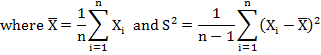
where S2 is an unbiased estimate of the population variance σ2, and it follows student’s t distribution with (n-1) degrees of freedom.
Therefore (n-1) S2=n s2
18.3 Applications of t-test
The t-test has number of applications in statistics which are discussed in following sections
· t-test for significance of single mean, population variance being unknown
· t-test for the significance of the difference between two means, the population variances being equal
· t-test for significance of an observed sample correlation coefficient.
18.3.1 t-Test for single mean
Suppose
we want to test
(i)
If
the given normal population has a specified value of the population mean μ0.
(ii) If
the sample mean differs from the specified value μ0 of the
population mean.
(iii) If
a random sample of size n viz., Xi (i=1,2,…, n) has been drawn from a normal population with
specified mean μ0.
Basically all the above three
problems are same with corresponding null hypothesis Ho as follows
(i)
µ
= μ0 i.e., the population mean is μ0
(ii) There
is no difference between the sample mean ![]() and the population
means μ.
and the population
means μ.
(iii) The
given sample has been drawn from the population with mean μ0
.
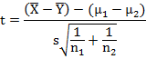
The test statistic is
given by


follows
student’s t distribution with (n-1) degrees of freedom. If calculated |t| >
tabulated value of t at 5 percent level of significance viz., t0.05;
(n-1) d.f. then Ho is rejected at 5 per
cent level of significance which implies that there is a significant difference
between sample mean and population mean or the sample has not been drawn from
the population having specified mean µ = μ0. If calculated |t|
< tabulated value of t at 5 percent level of significance viz., t0.05;
(n-1) d.f. then Ho is accepted. This
is explained with the help of following illustrations.
Example .1:
A random sample of 9 values from a normal population showed a mean of 41.5 and the
sum of squares of deviations from the mean equal to 72.Test whether the
assumption of mean 44.5 in the population is reasonable.
Solution: In this problem n=9 μ=44.5, ![]() =41.5 and
=41.5 and ![]()
H0: μ=44.5 i.e., population mean is 44.5
H1:
µ ≠ 44.5
Applying t-test

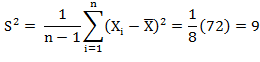
![]()
Tabulated value of t at 5% level of significance and 8 d.f. =2.306. Since the calculated value of |t| is greater than tabulated value 2.306, hence it is significant. We reject null hypothesis and conclude that the population mean is not equal to 44.5.
Example 2: An automatic machine was expected to fill 250 ml of flavored milk in the pouches. A random sample of pouches was taken and the actual content of milk was weighed. Weight of flavored milk (in ml.) is
253, 251, 248, 251, 252, 250, 249, 254, 247, 249, 248, 255, 245, 246, 254.
Do you consider that the average quantity of flavored milk in the sample is the same as that of adjusted value?
Solution : In this problem n=15 μ=250 ml.
H0: μ=250 ml i.e., automatic machine on an average fills 250 ml milk in each pouch
H1: µ ≠ 250
Prepare the following table
Table
18.1
|
Xi |
|
|
|
|
|
253 |
|
2.8667 |
|
8.2178 |
|
251 |
|
0.8667 |
|
0.7511 |
|
248 |
|
-2.1333 |
|
4.5511 |
|
251 |
|
0.8667 |
|
0.7511 |
|
252 |
|
1.8667 |
|
3.4844 |
|
250 |
|
-0.1333 |
|
0.0178 |
|
249 |
|
-1.1333 |
|
1.2844 |
|
254 |
|
3.8667 |
|
14.9511 |
|
247 |
|
-3.1333 |
|
9.8178 |
|
249 |
|
-1.1333 |
|
1.2844 |
|
248 |
|
-2.1333 |
|
4.5511 |
|
255 |
|
4.8667 |
|
23.6844 |
|
245 |
|
-5.1333 |
|
26.3511 |
|
246 |
|
-4.1333 |
|
17.0844 |
|
254 |
|
3.8667 |
|
14.9511 |
|
3752 |
|
0.0000 |
|
131.7333 |
![]()
Applying t-test
![]()
Tabulated value of t at 5% level of significance for 14 d.f. is 2.15. Since the calculated value of |t| is less than tabulated value 2.15, hence it is not significant. We accept null hypothesis and conclude that the on an average automatic machine fills 250 ml. of flavored milk in pouches.
18.3.2
t-Test for difference of means
Suppose
we want to test if two independent samples Xi (i=1,2,…,n1)
and Yj(j=1,2,…,n2) of sizes n1
and n2 have been drawn from two normal populations with means μ1
and μ2 respectively. Under the Null hypothesis Ho: µ1
= μ2 i.e. ,that the samples
have been drawn from the populations having same mean .
H1:
µ ≠ μ0
The t- statistic is given by
which
follows t distribution with (n1 + n2 -2)

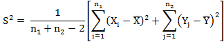
is an unbiased estimate of the common population variance σ2 based on both the samples. By comparing the computed value of t with the tabulated value of t for (n1 + n2 -2) d.f. and at desired level of significance, we reject or retain null hypothesis Ho
18.3.2.1 Assumptions for difference of means test
(i) Parent
populations from which the samples have been drawn are normally distributed.
(ii) The two samples are random and independent of
each other.
(iii) The population variances are equal σ12
= σ22 = σ2 but unknown.
Thus before applying t-test for testing the equality means, it is theoretical desirable to test the equality of population variances by applying F-test. If the hypothesis Ho: σ12 = σ22 is rejected then we cannot apply t-test and in such situations Behren’s d test is applied. This procedure is explained with the help of following illustrations.
Example 3 : The prices of ghee were compared in two cities. For this purpose ten shops were selected at random in each city. The following table gives per kg. prices of ghee in two cities:
|
City A |
361 |
363 |
356 |
364 |
359 |
360 |
362 |
361 |
358 |
357 |
|
City B |
368 |
369 |
370 |
366 |
367 |
365 |
371 |
372 |
366 |
367 |
Test whether the average price of ghee is of the same order in two cities.
Solution :
Null hypothesis Ho: µA=μB i.e., average price of ghee is of same order in cities A and B.
H1: µA ≠ μB
Prepare the following table:
Table 18.2
|
City A |
City B |
||||
|
Xi |
|
|
Yj |
|
|
|
361 |
0.9 |
0.81 |
368 |
-0.1 |
0.01 |
|
363 |
2.9 |
8.41 |
369 |
0.9 |
0.81 |
|
356 |
-4.1 |
16.81 |
370 |
1.9 |
3.61 |
|
364 |
3.9 |
15.21 |
366 |
-2.1 |
4.41 |
|
359 |
-1.1 |
1.21 |
367 |
-1.1 |
1.21 |
|
360 |
-0.1 |
0.01 |
365 |
-3.1 |
9.61 |
|
362 |
1.9 |
3.61 |
371 |
2.9 |
8.41 |
|
361 |
0.9 |
0.81 |
372 |
3.9 |
15.21 |
|
358 |
-2.1 |
4.41 |
366 |
-2.1 |
4.41 |
|
357 |
-3.1 |
9.61 |
367 |
-1.1 |
1.21 |
|
3601 |
60.9 |
3681 |
48.9 |
||
and
calculate,
![]()
![]()
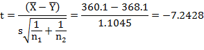
Tabulated value of t at 5% level of significance and 18 d.f. (for two–tail) is 2.10. Since the calculated value of |t| is more than tabulated value (2.10), hence it is significant. We reject null hypothesis at 5 percent level of significance and conclude that average prices of ghee in both the cities are different.
18.3.3 Paired t-test
Let us now consider the case when
(i) Sample sizes are equal i.e., n1 = n2 = n and
(ii) The samples are not independent but the sample observations are paired together i.e., the pair of observations (Xi, Yi) i=1,2,…,n corresponds to the same ith sample unit. The problem is to test if the sample means differ significantly or not.
For example suppose we want to test the efficacy of a particular drug say for inducing sleep or controlling blood pressure or blood sugar among the patients or if we want to test the difference between two analysts or machines with regard to detection of mean fat percentage in milk. Let Xi and Yi (i=1,2,…,n) be the readings of fat percentage of ith milk sample, detected by two machines A and B respectively. Here instead of applying the difference of the means test discussed in previous section, we apply paired t-test.
Here we consider the difference di = Xi – Yi (i=1,2,…,n)
Under the Null hypothesis Ho difference in fat percent in milk by both the machines is due to fluctuations of sampling i.e., H0: μd = 0
against H1: μd ≠ 0
then the test statistic
![]()
follows t distribution with (n-1) degrees of freedom

Different examples of paired t test are:
1. A sample of boys was given a test mathematics. They were given a month’s extra coaching and a second test was held at the end of it? Do the marks give evidence that the students have been benefitted by the extra coaching?
2. A sample of patients was examined to know whether a drug tends to reduce the blood pressure. The data give the blood pressure readings before the drug was given and also after it was given. The question is to examine whether the drug is effective in controlling blood pressure.
3. It is desired to test the adoption of a new technology by the farmers. A group of farmers is taken where the knowledge level score is measured before the new technology is infused and after infusion of technology, the knowledge level score is again measured. Do the difference in technology level scores provide the evidence that the farmers have been benefitted by the adoption of new technology.
This procedure is explained with the help of following illustrations.
Example 4:
Ten B.Tech. (Dairy Tech.) second year students were selected for a
training on quality control on the basis of marks obtained in an examination
conducted for this purpose . After one month training they were given a test
and marks were recorded out of 50.
|
Student |
A |
B |
C |
D |
E |
F |
G |
H |
I |
J |
|
Before
training |
25 |
20 |
35 |
15 |
42 |
28 |
26 |
44 |
35 |
48 |
|
After
training |
26 |
20 |
34 |
13 |
43 |
40 |
29 |
41 |
36 |
46 |
Test whether there is any change in performance
after the training.
Solution:
In this problem, the marks obtained by
the students before training (X) and after training (Y) are not independent but
paired together, hence we shall apply paired t test. Null Hypothesis
Ho: µX=μY
or H0: μd = 0 i.e.,
mean scores before training and after training are same .
In other words, the training has no impact on students’ performance
against H1: μd ≠ 0.
Preapare
the following table
Table 18.3
|
Before training (Xi) |
After training(Yi) |
di = Xi – Yi |
di2 |
|
25 |
26 |
-1 |
1 |
|
20 |
20 |
0 |
0 |
|
35 |
34 |
1 |
1 |
|
15 |
13 |
2 |
4 |
|
42 |
43 |
-1 |
1 |
|
28 |
40 |
-12 |
144 |
|
26 |
29 |
-3 |
9 |
|
44 |
41 |
3 |
9 |
|
35 |
36 |
-1 |
1 |
|
48 |
46 |
2 |
4 |
|
Total |
|
|
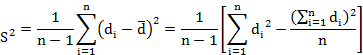
and calculate
![]()
![]()
Tabulated value of t at 5% level of significance and 9 d.f. (for two–tail) is 2.262. Since the calculated value of |t| is less than tabulated value 2.262, hence it is not significant. We accept null hypothesis and conclude that students have not been benefited from the training.
Example 5: A certain stimulus administered to each of 12 calves resulted in the following changes in the blood sugar levels 5, 2, 8,-1, 3,0, -2, 1, 5, 0, 4, 6 .
Can it be concluded that the stimulus will in general be accompanied by increase in blood sugar level? Test at 5% level of significance.
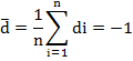
Solution: In this problem we are given the increments di =Xi –Yi in the blood sugar levels of 12 calves
Null Hypothesis Ho: µX=μY or μd = 0, i.e., there is no difference in blood sugar levels of the calves before and after the administering drug. In other words, the stimulus has no impact on blood sugar levels of calves.
Against H1: µX<μY or μd < 0 .i.e., the stimulus results in increase in blood sugar level of calves.
Preapare the following table:
|
di |
5 |
2 |
8 |
-1 |
3 |
0 |
-2 |
1 |
5 |
0 |
4 |
6 |
|
|
di2 |
25 |
4 |
64 |
1 |
9 |
0 |
4 |
1 |
25 |
0 |
16 |
6 |
|
and calculate
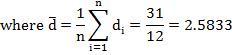
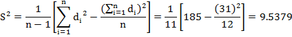
![]()
Tabulated value of t at 10% level of significance and 14 d.f. is 1.80 [in this problem the alternative hypothesis is right tailed hence to test at 5% level of significance we have to see the t table at 10% level of significance]. Since the calculated value of |t| is greater than tabulated value 1.80, hence it is significant. We reject null hypothesis and conclude that the stimulus is effective in increasing blood sugar in calves.
18.3.4 t-Test for significance of an observed sample correlation coefficient
Let a random sample (xi ,yi) (i=1,2---,n) of size n has been drawn from a bivariate normal distribution and let r be the observed sample correlation coefficient . In order to test whether sample correlation coefficient r is significant or there is no correlation between the variables in the population. Prof. R. A. Fisher proved that under the null hypothesis Ho: ρ=0 i.e. the population correlation coefficient is zero. The statistic
![]()
follows
student’s t distribution with (n-2) d.f., n being the
sample size.