Module 2. Linear
programming problem
Lesson 3
MATHEMATICAL FORMULATION OF THE LINEAR PROGRAMMING PROBLEM AND ITS GRAPHICAL SOLUTION
3.1 Introduction
A large number of business and economic situations are concerned with problems of planning and allocation of resources to various activities. In each case there are limited resources at our disposal and our problem is to make such a use of these resources so as to maximize production or to derive the maximum profit, or to minimize the cost of production etc. Such problems are referred to as the problems of constrained optimization. Linear programming (LP) is one of the most versatile, popular and widely used quantitative techniques. Linear Programming is a technique for determining an optimum schedule chosen from a large number of possible decisions. The technique is applicable to problem characterized by the presence of a number of decision variables, each of which can assume values within a certain range and affect their decision variables. The variables represent some physical or economic quantities which are of interest to the decision maker and whose domain are governed by a number of practical limitations or constraints which may be due to availability of resources like men, machine, material or money or may be due quality constraint or may arise from a variety of other reasons. The most important feature of linear programming is presence of linearity in the problem. The word Linear stands for indicating that all relationships involved in a particular problem are linear. Programming is just another word for “planning” and refers to the process of determining a particular plan of action from amongst several alternatives. The problem thus reduces to maximizing or minimizing a linear function subject to a number of linear inequalities
3.2 Definitions of Various Terms Involved in Linear Programming
3.2.1 Linear
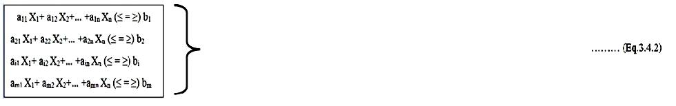
The word linear is used to describe the relationship among two or more variables which are directly proportional. For example, if the production of a product is proportionately increased, the profit also increases proportionately, then it is a linear relationship. A linear form is meant a mathematical expression of the type,
![]()
3.2.2 Programming
The term “Programming” refers to planning of activities in a manner that achieves some optimal result with resource restrictions. A programme is optimal if it maximizes or minimizes some measure or criterion of effectiveness, such as profit, cost or sales.
3.2.3 Decision variables and their relationship
The decision (activity) variables refer to candidates (products, services, projects etc.) that are competing with one another for sharing the given limited resources. These variables are usually inter-related in terms of utilisation of resources and need simultaneous solutions. The relationship among these variables should be linear.
3.2.4 Objective function
The Linear Programming problem must have a well defined objective function for optimization. For example, maximization of profits or minimization of costs or total elapsed time of the system being studied. It should be expressed as linear function of decision variables.
3.2.5 Constraints
There are always limitations on the resources which are to be allocated among various competing activities. These resources may be production capacity, manpower, time, space or machinery. These must be capable of being expressed as linear equalities or inequalities in terms of decision variables.
3.2.6 Alternative courses of action
There must be alternative courses of action. For example, there may be many processes open to a firm for producing a commodity and one process can be substituted for another.
3.2.7 Non-negativity restriction
All the variables must assume non-negative values, that is, all variables must take on values equal to or greater than zero. Therefore, the problem should not result in negative values for the variables.
3.2.8 Linearity and divisibility
All relationships (objective functions and constraints) must exhibit linearity, that is, relationships among decision variables must be directly proportional. For example, if our resources increase by some percentage, then it should increase the outcome by the same percentage. Divisibility means that the variables are not limited to integers. It is assumed that decision variables are continuous, i.e., fractional values of these variables must be permissible in obtaining an optimal solution.
3.2.9 Deterministic
In LP model (objective functions and constraints), it is assumed that the entire model coefficients are completely known (deterministic), e.g. profit per unit of each product, and amount of resources available are assumed to be fixed during the planning period.
3.3 Formulation of a Linear Programming Problem
The formulation of the Linear Programming Problem (LPP) as mathematical model involves the following key steps:
Step
1.
Identify the decision variables to be determined and express them in terms of
algebraic symbols as X1,X2, --- , Xn.
Step 2. Identify the objective which
is to be optimized (maximized or minimized) and express it as a linear function
of the above defined decision variables.
Step 3. Identify all the constraints in the given problem and then express them as linear equations or inequalities in terms of above defined decision variables.
Step 4. Non-negativity restrictions on decision variables.
The formulation of a linear programming problem can be illustrated through the following examples:
Example 1
A milk plant manufactures two types of products A and B and sells them at a profit of Rs. 5 on type A and Rs. 3 on type B. Each product is processed on two machines G and H. Type A requires one minute of processing time on G and two minutes on H; type B requires one minute on G and one minute on H. The machine G is available for not more than 6 hours 40 minutes, while machine B is available for 8 hours 20 minutes during any working day; formulate the problem as LP problem.
Solution
Let X1 be the number of products of type A and X2 the number of products of type B. Since the profit on type A is Rs. 5 per product, 5X1 will be the profit on selling X1units of type A. Similarly, 3X2 will be the profit on selling X2 units of type B. Therefore, total profit on selling X1 units of A and X2 units of B is given by Z = 5X1+3X2. Since this has to be maximized, hence the objective function can be expressed as
Max Z = 5X1+3X2 (Objective function)
Since machine G takes 1 minute time on type A and 1 minute time on type B, the total time in minutes required on machine G is given by X1+X2. Similarly the total time in minutes required on machine H is given by 2X1+X2. But machine G is not available for more than 6 hour 40 minutes (400 minutes), therefore
X1+X2 ≤ 400 (first constraint on machine G)
Also the machine H is available for 8
hours 20 minutes only, therefore
2X1+X2 ≤ 500 (second constraint on machine H)
Since it is not possible to produce
negative quantities,
X1 ≥0, X2 ≥0 (non-negativity restrictions)
Example 2
A dairy plant packs two types of milk in pouches viz., full cream and single toned. There are sufficient ingredients to make 20,000 pouches of full cream & 40,000 pouches of single toned. But there are only 45,000 pouches into which either of the products can be put. Further it takes three hours to prepare enough material to fill 1000 pouches of full cream milk & one hour for 1000 pouches of single toned milk and there are 66 hours available for this operation. Profit is Rs. 8 per pouch for full cream milk and Rs. 7 per pouch for single toned milk. Formulate it as a linear programming problem.
Solution
Let
number of full cream and single toned milk pouches to be packed is X1
and X2
Let
profit be Z
Objective
function: Max. Z = 8X1+7X2
Subject
to constraints: X1 + X2 ≤ 45000 (1)
X1 ≤ 20000 (2)
X2 ≤
40000 (3)
![]() (4)
(4)
Non-negativity restrictions X1,
X2 ≥0
Example 3
Consider two different types of food stuffs say F1 and F2. Assume that these food stuffs contain vitamin A and B. Minimum daily requirements of vitamin A and B are 40mg and 50mg respectively. Suppose food stuff F1 contains 2mg of vitamin A and 5mg of vitamin B while F2 contains 4mg of vitamin A and 2mg of vitamin B. Cost per unit of F1 is Rs. 3 and that of F2 is Rs. 2.5. Formulate the minimum cost diet that would supply the body at least the minimum requirements of each vitamin.
Solution
Let number of units needed for food stuffs F1 and F2 to meet the daily requirements of vitamins A and B be respectively X1 and X2..
Objective function: Minimize Z =3X1+2.5X2
Subject to constraints:
2X1+4X2 ≥ 40
5X1+2X2 ≥50
Non-negativity restrictions X1,
X2 ≥ 0
3.4 Mathematical Formulation of a General Linear Programming Problem
The general formulation of LP problem can be stated as follows. If we have n-decision variables X1, X2,…, Xn and m constraints in the problem , then we would have the following type of mathematical formulation of LP problem
Optimize
(Maximize or Minimize) the objective function:
Z = C1X1 + C2X2 + … + CnXn ……… (Eq.3.4.1)
Subject to
satisfaction of m- constraints:
Where the constraint may be in the form of an inequality (≤ or ≥) or even in the form of an equality (=) and finally satisfy the non-negativity restrictions
X1, X2, … , Xn ≥ 0 ……… (Eq.3.4.3)
where Cj (j=1, 2,….,n); bi (i=1, 2,…,m) and aij are all constants and m<n, and the decision variables Xj ≥0, j=1, 2,…,n. If bi is the available amount of resource i then aij is amount of resource i that must be allocated (technical coefficient) to each unit of activity j.
NOTE: By convention, the values of RHS parameters bi (i=1, 2, 3,…,m) are restricted to non-negative values only. If any value of bi is negative then it is to be changed to a positive value by multiplying both sides of the constraint by -1. This not only changes the sign of all LHS Coefficients and of RHS parameters but also changes the direction of inequality sign.
3.4.1 Matrix form of LP problem
The linear programming problem (3.4.1), (3.4.2) and (3.4.3) can be expressed in matrix form as
Maximize Z = CX
(objective
function )
Subject to AX = b, b ≥
0
(constraint
equation )
X ≥ 0 (non-negativity restriction )
Where X = (X1,X2, … , Xn), C = (C1,C2, … , Cn) and b = (b1,b2, … , bm)
3.5 Graphical Solution of Linear Programming Problem
LP problems which involve only two variables can be solved graphically. Such a solution by geometric method involving only two variables is important as it gives insight into more general case with any number of variables.
3.5.1 Feasible solution
A set value of the variables of a linear programming problem which satisfies the set of constraints and the non-negative restrictions is called feasible solution of the problem.
3.5.2 Feasible region
The collection of all feasible solutions is known as the feasible region. Any point which does not lie in the feasible region cannot be a feasible solution to the LP problems. The feasible region does not depend on the form of the objective function in any way. If we can represent the relations of the general LP problem on an n dimensional space, we will obtain a shaded solid figure (known as Convex-polyhedron) representing the domain of the feasible solution.
3.5.3 Optimal solution
A feasible solution of a linear programming problem which optimizes its objective function is called the optimal solution of the problem. Theoretically, it can be shown that objective function of a LP problem assumes its optimal value at one of the vertices (called extreme points) of this solid figure.
Steps to find graphical solution of the linear programming problem
Step 1: Formulate the linear programming problem.
Step 2: Draw the constraint equations on XY-plane.
Step 3: Identify the feasible region which satisfies all the constraints simultaneously. For less than or equal to constraints the region is generally below the lines and for greater than or equal to constraints, the region is above the lines.
Step 4: Locate the solution points on the feasible region. These points always occur at the vertices of the feasible region.
Step 5: Evaluate the optimum value of the objective function.
The geometric interpretation and solution for the LP problem using graphical method is illustrated with the help of following examples
Example 4 Find the graphical solution of problem formulated in example 1.
Max Z = 5X1+3X2
Subject to
X1+X2 ≤ 400
2X1+X2 ≤ 500
X1 ≥ 0 , X2 ≥0
Solution
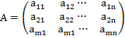
Any point lying in the first quadrant has X1, X2 ≥ 0 and hence satisfies the non-negativity restrictions. Therefore, any point which is a feasible solution must lie in the first quadrant. In order to find the set of points in the first quadrant which satisfy the constraints, we must interpret geometrically inequalities such as X1+X2≤ 400. If equality holds then we have the equation X1+X2= 400 i.e., any point on the straight line satisfies the equation. Any point lying on or below the line X1+X2= 400 satisfies the constraint X1+X2≤ 400. However, no point lying above the line satisfies the inequality. In a similar manner, we can find the set of points satisfying 2X1+X2 ≤ 500 and the non-negativity restrictions are all the points in the first quadrant. The set of points satisfying the constraints and the non-negativity restrictions is the set of points in the shaded region of the figure OABC as shown in Fig 3.1 Any point in this region is a feasible solution, and only the points in this region are feasible solutions. To solve the LP problem, we must find the point or points in the region of feasible solutions which give the largest value of the objective function. Now for any fixed value of Z, Z = 5X1+3X2 is a straight line, for each different values of Z, we obtain a different line. Again, all the lines corresponding to different values of Z are parallel; clearly our interest is to find the line with the largest value of Z which has at least one point in common with the region of feasible solutions. The line Z= 5X1+3X2 is drawn for various values of Z. It can be seen that the point farthest from Z = 5X1+3X2 and yet in the feasible region is B (100, 300) and thus point B maximizes Z while satisfying all the constraints. In other words, the corner B of the region of feasible solutions is the optimal solution of the LP problem. Since B is the intersection of the lines X1+X2=400 and 2X1+X2=500, it can be seen that at vertex B, X1=100 and X2=300. The maximum value of Z = 5(100)+3(300)=1400.The fact that the optimum occurred at the vertex B of the feasible region is not a coincidence but on the other hand represents a significant property of optimal solutions of all LP problems. To find the optimal solution find the values of objective function at the various extreme points as shown in the following Table 3.1
Table 3.1 Computation of maximum value of objective function
|
Extreme Point |
Coordinates |
Profit Function Z = 5X1+3X2 |
|
O |
X1=0 , X2=0 |
Z=5(0)+3(0)=0 |
|
A |
X1=0 , X2=400 |
Z=5(0)+3(400)=1200 |
|
B |
X1=100, X2=300 |
Z=5(100)+3(300)=1400 |
|
C |
X1=250, X2=0 |
Z=5(250)+3(0)=1250 |
Note: A fundamental theorem in LP states that the feasible region of any LP is a convex polygon (that is the n dimensional version of two dimensional polygon), with a finite number of vertices, and further for any LP problem, there is at least one vertex which provides an optimal solution. Whenever a LP problem has more than one optimal solution, we say that there are alternative optimal solutions. Physically, this means that the resources can be combined in more than one way to maximize profit.
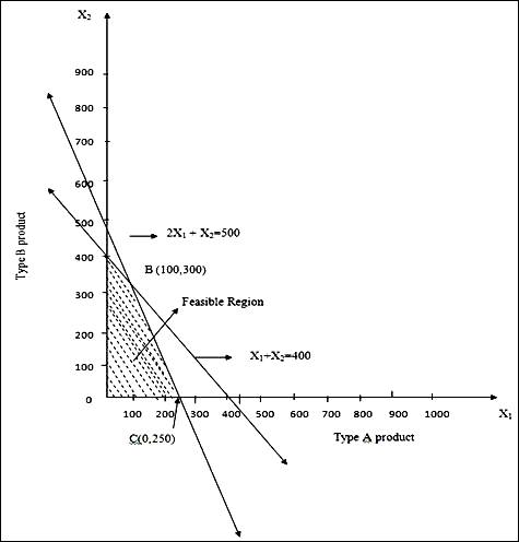
Fig. 3.1 Feasible region
Example 5 Find the graphical solution of problem formulated in Example 2.
Solution
Let number of full cream and single toned milk pouches to be produced is X1and X2 and Let profit be Z
Objective function: Max. Z = 8X1+7X2
Subject
to constraints: X1 + X2 ![]() 45000 (1)
45000 (1)
X1 ![]() 20000 (2)
20000 (2)
X2 ![]() 40000 (3)
40000 (3)
3X1 + X2 ![]() 66000 (4)
66000 (4)
Non-negativity
restrictions X1, X2![]() 0
0
First of all draw the graphs of these inequalities (as discussed in Example 5) which is shown in Fig. 3.2.
Fig. 3.2 Feasible region
To find the optimal solution find the values of objective function at the various extreme points as shown in the following Table 3.2
Table 3.2 Computation of maximum value of objective function
|
Extreme Point |
Coordinates |
Profit Function Z = 8X1+7X2 |
|
O |
X1=0 , X2=0 |
Z=8(0)+7(0)=0 |
|
A |
X1=0 , X2=40000 |
Z=8(0)+7(40000)=280000 |
|
B |
X1=5000, X2=40000 |
Z=8(5000)+7(40000)=320000 |
|
C |
X1=10500, X2=34500 |
Z=8(10500)+7(34500)=325500 |
|
D |
X1=20000 , X2=6000 |
Z=8(20000)+7(6000)=202000 |
|
E |
X1=20000 , X2=0 |
Z=8(20000)+7(0)=160000 |
So maximum value of Z occurs at point C (10500, 34500) so it is the optimal solution. It can be concluded that Dairy Plant must produce 10500 pouches of full cream milk and 34500 pouches of single toned milk.
Let us consider the following example to illustrate graphical solution for minimization problem
3.5.4 Special cases in linear programming
Up till now we have discussed those problems which have a unique optimal solution. However, it is possible for LP problem to have following special cases.
3.5.4.1
Unbounded solution
A linear programming problem is considered to have an unbounded solution if it has no limits on the constraints and further, the common feasible region is not bounded in any respect.
Example 6 Find the graphical solution of problem formulated in example 3.
Solution
Let number of units needed for food stuffs F1 and F2 to meet the daily requirements of vitamins A and B be respectively X1 and X2..
Objective function: Minimize Z = 3X1+2.5X2
Subject to constraints: 2X1+4X2 ≥ 40
5X1+2X2 ≥50
Non-negativity restrictions: X1,
X2![]() 0
0
First of all draw the graphs of these inequalities (as discussed in example 5) .Since the inequalities are of the greater than or equal to type, the feasible region is formed by considering the area to the upper right side of each equation i.e. away from origin .The shaded area which is shown above CBD is satisfied by the two constraints as shown in Fig. 3.3 is feasible region. The feasible region for minimization problem is unbounded and unlimited. Since the optimal solution corresponds to one of the corner (extreme) points, we will calculate the values of objective function for each corner point viz. D (20, 0); B (7.5, 6.25) and C (0, 25). The calculations are shown in Table 3.3
Table 3.3 Table showing the computation of minimum value of objective function
|
Extreme Point |
Coordinates |
Cost Function Min. Z = 3X1+2.5X2 |
|
D |
X1=20 , X2=0 |
Z=3(20)+2.5(0)=60 |
|
B |
X1=7.5 , X2=6.25 |
Z=3(7.5)+2.5(6.25)=38.125 |
|
C |
X1=0, X2=25 |
Z=3(0)+2.5(25)=62.5 |

Fig. 3.3 Feasible region for minimization problem
The minimum cost is obtained at the corner point B(7.5,6.25) i.e. X1=7.5 and X2=6.25. Hence to minimize the cost and to meet the daily requirements of vitamin A and B, number of units needed of food stuffs F1 and F2 be 7.5 and 6.25 respectively.
3.5.5 Infeasible solution
In this there is no solution to an LP Problem that satisfies all the constraints. Graphically, it means that no feasible solution region exists. Such a condition indicates that the LP problem has been wrongly formulated.
3.5.6 Redundant constraint
In a properly formulated LP problem, each of the constraints will define a portion of the boundary of the feasible solution region. Whenever, a constraint does not define a portion of the boundary of the feasible solution region, it is called a redundant constraint. Let us consider the following example to illustrate this.
Example 7 Maximize Z=1170X1+1110X2
Subject to:
|
9X1+5X2 ≥ 500 |
|
7X1+9X2 ≥ 300 |
|
5X1+3X2 ≤ 1500 |
|
7X1+9X2 ≤1900 |
|
2X1+4X2 ≤ 1000 |
|
X1, X2
≥
0 |
The
feasible region of this LP problem is indicated in Fig. 2.4. In this the
feasible region has been formulated by two constraints.
9X1+5X2 ≥ 500
7X1+9X2 ≤1900
X1, X2 ≥ 0
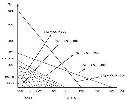
Fig 3.4 Feasible Region and Redundant Constraints
The remaining three constraints, although present, is not affecting the feasible region in any manner. Such constraints are known as redundant constraints.