Module 4. Assignment problem
Lesson 9
SOLUTION OF ASSIGNMENT PROBLEM
9.1 Introduction
Although assignment problem can be solved either by using the techniques of Linear Programming or by the transportation method yet the assignment method developed by D. Konig, a Hungarian mathematician known as the Hungarian method of assignment problem is much faster and efficient. In order to use this method, one needs to know only the cost of making all the possible assignments. Each assignment problem has a matrix (table) associated with it. Normally, the objects (or people) one wishes to assign are expressed in rows, whereas the columns represent the tasks (or things) assigned to them. The number in the table would then be the costs associated with each particular assignment. It may be noted that the assignment problem is a variation of transportation problem with two characteristics firstly the cost matrix is a square matrix and secondly the optimum solution for the problem would be such that there would be only one assignment in a row or column of the cost matrix.
9.2 Solution of Assignment Problem
The assignment problem can be solved by the following four methods:
a) Complete enumeration method
b) Simplex Method
c) Transportation method
d) Hungarian method
9.2.1 Complete enumeration method
In this method, a list of all possible assignments among the given resources and activities is prepared. Then an assignment involving the minimum cost, time or distance or maximum profits is selected. If two or more assignments have the same minimum cost, time or distance, the problem has multiple optimal solutions. This method can be used only if the number of assignments is less. It becomes unsuitable for manual calculations if number of assignments is large
9.2.2 Simplex method
This can be solved as a linear programming problem as discussed in section 8.1.3 of the last lesson and as such can be solved by the simplex algorithm.
9.2.3 Transportation method
As assignment is a special case of transportation problem, it can also be solved using transportation model discussed in module 3. The solution obtained by applying this method would be degenerate. This is because the optimality test in the transportation method requires that there must be m+n-1= (2n-1) basic variables. For an assignment problem of order n x n there would be only n basic variables in the solution because here n assignments are required to be made. This degeneracy problem of solution makes the transportation method computationally inefficient for solving the assignment problem.
9.2.4 Hungarian assignment method
The Hungarian method of assignment provides us with an efficient means of finding the optimal solution. The Hungarian method is based upon the following principles:
(i) If a constant is added to every element of a row and/or column of the cost matrix of an assignment problem the resulting assignment problem has the same optimum solution as the original problem or vice versa.
(ii) The solution having zero total cost is considered as optimum solution.
Hungarian method of assignment problem (minimization case) can be summarized in the following steps:
Step I: Subtract the minimum cost of each row of the cost (effectiveness) matrix from all the elements of the respective row so as to get first reduced matrix.
Step II: Similarly subtract the minimum cost of each column of the cost matrix from all the elements of the respective column of the first reduced matrix. This is first modified matrix.
Step III: Starting with row 1 of the first modified matrix, examine the rows one by one until a row containing exactly single zero elements is found. Make any assignment by making that zero in or enclose the zero inside a. Then cross (X) all other zeros in the column in which the assignment was made. This eliminates the possibility of making further assignments in that column.
Step IV: When the set of rows have been completely examined, an identical procedure is applied successively to columns that is examine columns one by one until a column containing exactly single zero element is found. Then make an experimental assignment in that position and cross other zeros in the row in which the assignment has been made.
Step V: Continue these successive operations on rows and columns until all zeros have been either assigned or crossed out and there is exactly one assignment in each row and in each column. In such case optimal assignment for the given problem is obtained.
Step VI: There may be some rows (or columns) without assignment i.e. the total number of marked zeros is less than the order of the matrix. In such case proceed to step VII.
Step VII: Draw the least possible number of horizontal and vertical lines to cover all zeros of the starting table. This can be done as follows:
1. Mark (√) in the rows in which assignments has not been made.
2. Mark column with (√) which have zeros in the marked rows.
3. Mark rows with (√) which contains assignment in the marked column.
4. Repeat 2 and 3 until the chain of marking is completed.
5. Draw straight lines through marked columns.
6. Draw straight lines through unmarked rows.
By this way we draw the minimum number of horizontal and vertical lines necessary to cover all zeros at least once. It should, however, be observed that in all n x n matrices less than n lines will cover the zeros only when there is no solution among them. Conversely, if the minimum number of lines is n, there is a solution.
Step VIII: In this step, we
1. Select the smallest element, say X, among all the not covered by any of the lines of the table; and
2.
Subtract
this value X from all of the elements in the matrix not covered by lines and
add X to all those elements that lie at the intersection of the horizontal and
vertical lines, thus obtaining the second modified cost matrix.
Step IX: Repeat
Steps IV, V and VI until we get the number of lines equal to the order of
matrix I, till an optimum solution is attained.
Step X: We
now have exactly one encircled zero in each row and each column of the cost
matrix. The assignment schedule corresponding to these zeros is the optimum
assignment. The above technique is explained by taking the following examples
Example 1
A plant manager has four subordinates, and four tasks to be performed. The subordinates differ in efficiency and the tasks differ in their intrinsic difficulty. This estimate of the times each man would take to perform each task is given in the effectiveness matrix below.
|
|
I |
II |
III |
IV |
|
A |
8 |
26 |
17 |
11 |
|
B |
13 |
28 |
4 |
26 |
|
C |
38 |
19 |
18 |
15 |
|
D |
19 |
26 |
24 |
10 |
How should the tasks be allocated, one to a man, so as to minimize the total man hours?
Solution
Step I : Subtracting the smallest element in each row from every element in that row, we get the first reduced matrix.
|
0 |
18 |
9 |
3 |
|
9 |
24 |
0 |
22 |
|
23 |
4 |
3 |
0 |
|
9 |
16 |
14 |
0 |
Step II: Next, we subtract the smallest element in each column from every element in that column; we get the second reduced matrix.
Step III: Now we test whether it is possible to make an assignment using only zero distances.
|
0 |
14 |
9 |
3 |
|
9 |
20 |
0 |
22 |
|
23 |
0 |
3 |
0 |
|
9 |
12 |
14 |
0 |
(a) Starting with row 1 of the matrix, we examine rows one by one until a row containing exactly single zero elements are found. We make an experimental assignment (indicated by) to that cell. Then we cross all other zeros in the column in which the assignment was made.
(b) When the set of rows has been completely examined an identical procedure is applied successively to columns. Starting with Column 1, we examine columns until a column containing exactly one remaining zero is found. We make an experimental assignment in that position and cross other zeros in the row in which the assignment was made. It is found that no additional assignments are possible. Thus, we have the complete ‘Zero assignment’,
A – I, B – III, C – II, D – IV
The minimum total man hours are computed as
|
Optimal assignment |
Man hours |
|
A – I |
8 |
|
B – III |
4 |
|
C – II |
19 |
|
D – IV |
10 |
|
Total |
41 hours |
Example 2
A dairy plant has five milk tankers I, II, III, IV & V. These milk tankers are to be used on five delivery routes A, B, C, D, and E. The distances (in kms) between dairy plant and the delivery routes are given in the following distance matrix
|
|
I |
II |
III |
IV |
V |
|
A |
160 |
130 |
175 |
190 |
200 |
|
B |
135 |
120 |
130 |
160 |
175 |
|
C |
140 |
110 |
155 |
170 |
185 |
|
D |
50 |
50 |
80 |
80 |
110 |
|
E |
55 |
35 |
70 |
80 |
105 |
How the milk tankers should be assigned to the chilling centers so as to minimize the distance travelled?
Solution
Step I: Subtracting minimum element in each row we get the first reduced matrix as
|
30 |
0 |
45 |
60 |
70 |
|
15 |
0 |
10 |
40 |
55 |
|
30 |
0 |
45 |
60 |
75 |
|
0 |
0 |
30 |
30 |
60 |
|
20 |
0 |
35 |
45 |
70 |
Step II: Subtracting minimum element in each column we get the second reduced matrix as
|
30 |
0 |
35 |
30 |
15 |
|
15 |
0 |
0 |
10 |
0 |
|
30 |
0 |
35 |
30 |
20 |
|
0 |
0 |
20 |
0 |
5 |
|
20 |
0 |
25 |
15 |
15 |
Step
III: Row 1 has a single zero in column 2. We make an
assignment by putting ‘ ‘around it and delete other zeros in column
2 by marking ‘X’. Now column1 has a single zero in column 4 we make an assignment
by putting ‘ ‘and cross the other zero which is not yet crossed.
Column 3 has a single zero in row 2; we make an assignment and delete the other
zero which is uncrossed. Now we see that there are no remaining zeros; and row
3, row 5 and column 4 has no assignment. Therefore, we cannot get our desired
solution at this stage.
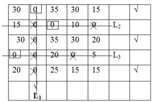
Step IV: Draw the minimum number of horizontal and vertical lines necessary to cover all zeros at least once by using the following procedure
1. Mark (√) row 3 and row 5 as having no assignments and column 2 as having zeros in rows 3 and 5.
2. Next we mark (√) row 2 because this row contains assignment in marked column 2. No further rows or columns will be required to mark during this procedure.
3. Draw line L1 through marked col.2.
4. Draw lines L2 & L3 through unmarked rows.
Step V: Select the smallest element say X among all uncovered elements which is X = 15. Subtract this value X=15 from all of the values in the matrix not covered by lines and add X to all those values that lie at the intersections of the lines L1, L2 & L3.
Applying these two rules, we get a new matrix
|
15 |
0 |
20 |
15 |
0 |
|
15 |
15 |
0 |
10 |
0 |
|
15 |
0 |
20 |
15 |
5 |
|
0 |
15 |
20 |
0 |
5 |
|
5 |
0 |
10 |
0 |
0 |
Step VI: Now
reapply the test of Step III to obtain the desired solution.
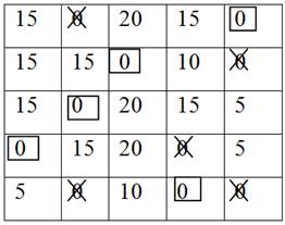
The assignments are
![]()
Total Distance
200 + 130 + 110 + 50 + 80 = 570