Module
3. Inventory control
Lesson 11
ECONOMIC LOT SIZE MODELS WITH KNOWN DEMAND
11.1 Introduction
In the last lesson we have seen that maintenance of proper Inventory Control System helps in keeping the investment in Inventories as low as possible and yet (i) ensures availability of materials by providing adequate protection against supply uncertainty and consumption of materials and (ii) allows full advantages of economies of bulk purchases and transportation costs. The basic Inventory Control problem therefore lies in determining firstly when should an order for materials be placed and secondly how much should be produced at the beginning of each time interval or what quantity of an item should be ordered each time. In this lesson we will learn how to develop inventory model.
11.2 Variables in Inventory Problem
The variables used in any inventory model are of two types: Controlled and Uncontrolled variables
11.2.1 Controlled variables
The following are the variables that may be considered separately or in combination:
· How much quantity acquired
· The frequency or timing of acquisition .How often or when to replenish the inventory?
· The completion stage of stocked items.
11.2.2 Uncontrolled variables
The following are the principal variables that may be controlled:
· The holding costs, shortage or penalty cost, set up costs.
· Demand: It is the number of units required per period and may be either known exactly or is known in terms of probabilities or is completely unknown. Further if the demand is known, it may be either fixed or variable per unit of time. The model which has fixed demand is known as deterministic model.
· Lead Time: This is the time of placing an order and its arrival in stock as shown in Fig. 11.1. If the lead time is known and not equal to zero and if demand is deterministic then one should order in advance by an amount of time equal to lead time. If the lead time is zero then there is no need to order in advance. If lead time is variable then it is known as probabilistically.
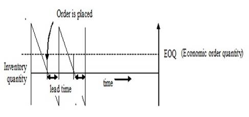
Fig. 11.1 Inventory with constant demand rate and constant lead time
· Amount delivered (supply of goods) : The supply of goods may be instantaneous or spread over a period of time .If a quantity q is ordered for purchase, the amount delivered may very around g with known probability density function .
11.3
Symbols Used in Inventory Models
C1 = Holding cost per
item per unit time
C2 = Shortage cost per
unit quantity per unit time for the back-log case and per unit only for no back log case.
C3 = Set up cost per
production run
R = Demand Rate
K = Production Rate
t = Scheduling time period which is
not prescribed.
tp = Scheduling time
period (prescribed)
z = Order Level (or stock level)
D = Total Demand
Q = Quantity already present in the
beginning
L = Lead time
11.4 Classification of Inventory Models
The inventory models are broadly classified as either deterministic (variables are known with certainty) or stochastic (variables are probabilistic). The deterministic models are further divided into Static demand models and dynamic demand models. In this lesson we will discuss deterministic inventory model i.e. economic lot size system with uniform demand.
11.5 Economic Order Quantity (EOQ) Model
This concept was developed by F. Haris in 1916. The concept is as lot size (q) increases the carrying charges (C1) will increase while the ordering cost (C3) will decrease. On the other hand as the lot size (q) decreases, the carrying cost (C1) will decrease but the ordering costs will increase. Economic Ordering Quantity (EOQ) is the size of order which minimizes total annual cost of carrying inventory and cost of ordering under the assumed conditions of certainly and annual demands are known.
11.5.1 The economic lot size system with uniform demand
In this model we want to derive an Economic Lot Size Formula for the optimum production quantity q per cycle (per production run) of a single product so as to minimize the total average variable cost per unit time. The model is based on the following basic assumptions:
i) The demand for the item is uniform at the rate of R quantity units per unit time
ii) The lead time is known and fixed. Thus, when the lead time is zero, the delivery of item is instantaneous.
iii) Production rate is infinite i.e. production is instantaneous
iv) Shortages are not allowed
v) Holding cost is Rs. C1 in per quantity unit per unit time
vi) Set up cost is Rs. C3 per set up.
This can be solved by two following methods
11.5.1.1 Algebraic method
The algebraic method is based on the following principle:
Inventory carrying
costs=Annual ordering (set up) costs
………
(Eq. 11.1)
Since the demand is uniform and known exactly and supply is instantaneous, the reorder point is that when inventory falls to zero.
Average Inventory =1/2(maximum level +minimum level) = (q+0)/2=q/2
Total inventory
carrying costs are determined by using the following formula:
(Total
inventory carrying costs per unit) = (average no. of units in inventory) × (costs of one unit)
×
(inventory carrying costs percentage) =1/2q×C×I=1/2qC1 ……… (Eq. 11.2)
Where C1 = CI is holding or carrying cost per unit for unit time.
Total annual ordering costs are obtained
as follows:
Total annual ordering costs =
(number of orders per year) ×
(ordering cost per order) = (R/q) ×
C3 = (R/q) C3 ………(Eq. 11.3)
Now summing up the total inventory
carrying cost and total ordering cost we get total inventory
cost as
Total ordering costs = (Total inventory carrying costs per unit) + (Total annual ordering costs)
C(q)= 1/2qC1+(R/q)C3 , this is cost equation . ………(Eq. 11.4)
The total inventory cost C(q) is minimum when the inventory carrying costs become equal to the total ordering costs. Therefore
1/2qC1=(R/q)C3
or ![]() ………(Eq. 11.5)
………(Eq. 11.5)
Or
optimal ![]()
To find the minimum of total inventory
cost C(q) , we substitute the value of q from (11.5) in cost equation
(11.4) we get
![]() ……… (Eq. 11.6)
……… (Eq. 11.6)
Optimum
inventory cost (Cmin) = ![]()
To obtain the optimum interval of
ordering (t*) we have
(Economic ordering quantity) = (demand rate) × (interval of ordering)
q = R × t
………
(Eq. 11.7)
![]() ……… (Eq. 11.8)
……… (Eq. 11.8)
11.5.1.2 Calculus method
Let each production cycle be made at
fixed interval‘t’ and therefore the quantity q already present in the beginning
(when the business was started) should be
Q = R.t ……… (Eq. 11.9)
where R is the demand rate.
Since the stock in small time dt will be
Rt.dt, therefore the stock in total time t will be ![]() =Area of the inventory ∆POA as shown in
Fig. 11.2
=Area of the inventory ∆POA as shown in
Fig. 11.2
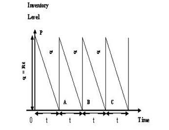
Fig. 11.2 Inventory profile of EOQ model
q
= Rt
The rate of replenishment = slope of
line ![]()
Thus the cost of holiday inventory is =
c1(Area of ∆OPA)
per production run
![]() ……… (Eq. 11.10)
……… (Eq. 11.10)
Set up cost is C3
per production run for interval
t.
……… (Eq. 11.11)
Total
cost C(t) is summing up the costs in (11.10) and (11.11) and dividing by t we
get the average total cost given by
![]() ………(Eq. 11.12)
………(Eq. 11.12)
The condition for minimum or maximum of C(t) is
![]()
![]() ……… (Eq. 11.13)
……… (Eq. 11.13)
![]()
![]()
![]() ………(Eq. 11.14)
………(Eq. 11.14)
![]() ……… (Eq. 11.15)
……… (Eq. 11.15)
which is known as optimal lot size formula.Therefore
per unit time is obtained by putting in equation (11.12).The above procedure is illustrated through following examples
Example 1 A manufacture has to supply his customer with 600 units of a product per year, shortages are not allowed and the storage costs amounts to 0.60 per unit per year. The set up cost per run is Rs. 80.00. Find the optimum run size and the minimum average yearly cost.
Solution
In this the demand rate (R) =600 per
unit per year
C1
= Holding cost per item per unit time = Rs. 0.60 per unit per year
C3 = Set up cost per production run = Rs. 80 per production run
Optimum
lot size is ![]()
= 0.67 years = 8 months
Thus the manufacturer should produce 400 units of his product at an interval of 8 months.
Example 2 A company uses 3000 units of a product, its carrying cost is 30%of average inventory. Ordering cost is Rs. 100 per order. Unit cost is Rs. 20.Calculate EOQ and the total cost.
Solution
D = Total Demand=3000 units
C1 = carrying cost =30%
of Rs. 20=Rs.6
C3 = Ordering cost =Rs.100
Optimum
lot size is ![]()
The total cost is equal to
Total cost = Material cost + Total
variable cost
![]()
![]()
11.6 Limitations of EOQ Formulae
In spite of several assumptions made in the derivation of above EOQ formulae, following are the limitations while considering applications of these formulae:
i) In the EOQ model we assumed that the demand for the item under consideration is constant, while in practical situations demand is neither known with certainty nor it is uniform.
ii) It is difficult to measure the ordering cost and also it is not linearly related to number of orders.
iii) In EOQ model it is assumed that the annual demand can be estimated in advance which is just a guess in practice.
iv) In EOQ model it is assumed that the entire inventory which is ordered arrives simultaneously. In many situations it may not be true.
v) In EOQ, it is assumed that the demand is uniform; which may not hold in practice.
vi) In
EOQ model, the replenishment time is assumed to be zero which is not possible
in real life always.