Module 8. Electric power economics
Lesson 31
MAXIMUM DEMAND CHARGE
31.1 Important Terms and Definitions
31.1.1 Demand
The rate at which electric energy is used in any instant or average over a period of time. Usually expressed in kilowatts (kW) or kilovolt-amperes (kVA).
31.1.2 Kilovolt amperes (kVA)
A measure of electrical load on a circuit or system. This unit is used to measure apparent electric power. For billing purposes maximum demand measured in kilowatts (kW) is converted to kilovolt amperes (kVA) by dividing by the power factor. Maximum demand and capacity charges are billed using kVA rather than kW.
31.1.3 Kilowatt
A measure of electrical power. One kilowatt (kW) equals 1,000 watts.
31.1.4 Kilowatt hour
A measure of electrical energy. One kilowatt hour (kWh) of energy is the energy produced by one kilowatt acting for one hour. Electricity meters record in kilowatt hours and electrical consumption is billed on kilowatt hours.
31.1.5 Load factor
Ratio of average energy demand (load) to maximum demand (peak load) during a specific period. Usually stated as a percentage, or number of hours used.
31.1.6 Maximum demand (MD)
The measure of the highest peak of electricity flow into the site during a half-hour period, in the period of a month. Measured in either kW or kVA.
31.1.7 Power factor
The ratio of active or real power in kilowatts (kW), to apparent power in kilovolt amperes or
kVA. Power Factor is normally expressed as a figure between zero and one. Unity power factor is 100% (or 1.0) power factor which is the highest available. In practice 0.99 is the highest.
31.1.8 Trivector meter
Trivector meter can measure active power, reactive power, apparent power i.e. with the help of a single meter we can measure kVA, kW, kVAR. The power triangle is sum of (kW, kVAR, kVA) and the meter which gives readings all of the above variables is called TRI vector meter.
31.2 Billing of Electricity
The electricity billing by utilities for medium & large enterprises, in High Tension (HT) category, is often done on two-part tariff structure, i.e. one part for capacity (or demand) drawn and the second part for actual energy drawn during the billing cycle. Capacity or demand is in kVA (apparent power) or kW terms. The reactive energy (i.e.) kVArh drawn by the service is also recorded and billed for in some utilities, because this would affect the load on the utility. Accordingly, utility charges for maximum demand, active energy and reactive power drawn (as reflected by the power factor) in its billing structure. In addition, other fixed and variable expenses are also levied. The tariff structure generally includes the following components:
a) Maximum demand Charges
These charges relate to maximum demand registered during month/billing period and corresponding rate of utility.
b) Energy Charges
These charges relate to energy (kilowatt hours) consumed during month / billing period and corresponding rates, often levied in slabs of use rates. Some utilities now charge on the basis of apparent energy (kVAh), which is a vector sum of kWh and kVArh.
c) Power factor penalty or bonus rates, as levied by most utilities, are to contain reactive power drawn from grid.
d) Fuel cost adjustment charges as levied by some utilities are to adjust the increasing fuel expenses over a base reference value.
e) Electricity duty charges levied w.r.t units consumed.
f) Meter rentals
g) Lighting and fan power consumption is often at higher rates, levied sometimes on slab basis or on actual metering basis.
h) Time of Day (TOD) rates like peak and non-peak hours are also prevalent in tariff structure provisions of some utilities.
i) Penalty for exceeding contract demand
j) Surcharge if metering is at LT side in some of the utilities
Analysis of utility bill data and monitoring its trends helps energy manager to identify ways for electricity bill reduction through available provisions in tariff framework, apart from energy budgeting. The utility employs an electromagnetic or electronic trivector meter, for billing purposes. The minimum outputs from the electromagnetic meters are
• Maximum demand registered during the month, which is measured in preset time intervals (say of 30 minute duration) and this is reset at the end of every billing cycle.
• Active energy in kWh during billing cycle
• Reactive energy in kVARh during billing cycle and
• Apparent energy in kVAh during billing cycle
It is important to note that while maximum demand is recorded, it is not the instantaneous demand drawn, as is often misunderstood, but the time integrated demand over the predefined recording cycle. As example, in an industry, if the drawl over a recording cycle of 30 minutes is:
250 kVA for 4 minutes
360 kVAfor 12 minutes
410 kVAfor 6 minutes
380 kVA for 8 minutes
The MD recorder
will be computing MD as:
![]()
The month’s maximum demand will be the highest among such demand values recorded over the month. The meter registers only if the value exceeds the previous maximum demand value and thus, even if, average maximum demand is low, the industry / facility has to pay for the maximum demand charges for the highest value registered during the month, even if it occurs for just one recording cycle duration i.e., 30 minutes during whole of the month. A typical demand curve is shown in Figure 31.1 the demand varies from time to time.
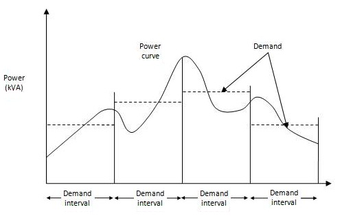
Fig. 31.1 Maximum demand curve
As can be seen from the Figure 31.1 the demand is measured over predetermined time interval and averaged out for that interval as shown by the horizontal dotted line. Fig. 31.2 shows the peak demand during 24 hour operation of a plant.
Fig. 31.2 Peak demand during a 24 hour operation
Most electricity boards have changed over from conventional electromechanical trivector meters to electronic meters, which have some excellent provisions that can help the utility as well as the industry. These provisions include:
• Substantial memory for logging and recording all relevant events
• High accuracy up to 0.2 class
• Amenability to time of day tariffs
• Tamper detection /recording
• Measurement of harmonics and Total Harmonic Distortion (THD)
• Long service life due to absence of moving parts
• Amenability for remote data access/downloads
Trend analysis of purchased electricity and cost components can help the industry to identify key result areas for bill reduction within the utility tariff available framework along the following lines.
Table 31.1 Purchased electrical energy trend
|
|
||||||||||
|
Month & Year |
MD Recorded kVA |
Billing Demand* kVA |
Total Energy Consumption kWh |
Energy Consumption During Peak Hours (kWh) |
MD Charge Rs./kVA |
Energy Charge Rs./kWh |
PF |
PF Penalty/ Rebate Rs. |
Total Bills Rs. |
Average Cost Rs./kWh |
|
Jan. |
|
|
|
|
|
|
|
|
|
|
|
Feb. |
|
|
|
|
|
|
|
|
|
|
|
|
|
|
|
|
|
|
|
|
|
|
|
|
|
|
|
|
|
|
|
|
|
|
|
|
|
|
|
|
|
|
|
|
|
|
|
Dec. |
|
|
|
|
|
|
|
|
|
|
31.3 Need for Electrical Load Management
In a macro perspective, the growth in the electricity use and diversity of end use segments in time of use has led to shortfalls in capacity to meet demand. As capacity addition is costly and only a long time prospect, better load management at user end helps to minimize peak demands on the utility infrastructure as well as better utilization of power plant capacities.
The utilities (State Electricity Boards) use power tariff structure to influence end user in better load management through measures like time of use tariffs, penalties on exceeding maximum demand, night tariff concessions etc. Load management is a powerful means of efficiency improvement both for end user as well as utility.
As the demand charges constitute a considerable portion of the electricity bill, from user angle too there is a need for integrated load management to effectively control the maximum demand.
31.4 Step by Step Approach for Maximum Demand Control
31.4.1 Load curve generation
Presenting the load demand of a consumer against time of the day is known as a ‘load curve’. If it is plotted for the 24 hours of a single day, it is known as an ‘hourly load curve’ and if daily demands plotted over a month, it is called daily load curves. A typical hourly load curve for an engineering industry is shown in Figure 31.3. These types of curves are useful in predicting patterns of drawl, peaks and valleys and energy use trend in a section or in an industry or in a distribution network as the case may be.
Fig. 31.3 Hourly load curve
31.4.2 Rescheduling of loads
Rescheduling of large electric loads and equipment operations, in different shifts can be planned and implemented to minimize the simultaneous maximum demand. For this purpose, it is advisable to prepare an operation flow chart and a process chart. Analyzing these charts and with an integrated approach, it would be possible to reschedule the operations and running equipment in such a way as to improve the load factor which in turn reduces the maximum demand.
31.4.3 Storage of Products/in process material/ process utilities like refrigeration
It is possible to reduce the maximum demand by building up storage capacity of products/ materials, water, chilled water / hot water, using electricity during off peak periods. Off peak hour operations also help to save energy due to favorable conditions such as lower ambient temperature etc. Example: Ice bank system is used in milk & dairy industry. Ice is made in lean period and used in peak load period and thus maximum demand is reduced.
31.4.4 Shedding of non-essential loads
When the maximum demand tends to reach preset limit, shedding some of non-essential loads temporarily can help to reduce it. It is possible to install direct demand monitoring systems, which will switch off non-essential loads when a preset demand is reached. Simple systems give an alarm, and the loads are shed manually. Sophisticated microprocessor controlled systems are also available, which provide a wide variety of control options like:
· Accurate prediction of demand
· Graphical display of present load, available load, demand limit
· Visual and audible alarm
· Automatic load shedding in a predetermined sequence
· Automatic restoration of load
· Recording and metering
31.4.5 Operation of captive generation and diesel generation sets
When diesel generation sets are used to supplement the power supplied by the electric utilities, it is advisable to connect the D.G. sets for durations when demand reaches the peak value. This would reduce the load demand to a considerable extent and minimize the demand charges.
31.4.6 Reactive power compensation
The maximum demand can also be reduced at the plant level by using capacitor banks and maintaining the optimum power factor. Capacitor banks are available with microprocessor based control systems. These systems switch on and off the capacitor banks to maintain the desired Power factor of system and optimize maximum demand thereby.
31.5 Electrical energy conservation in dairy processing plant
|
1. Power System · Transformer loading · Determination of plant load & load factor analysis · Improving power factor · Identification and minimsing transformer and system distribution losses · Demand management & controls · Parallel operation of DG/TG sets with grid · Use of harmonic filters near equipments generating harmonics to reduce total harmonic distortion
|
4. Refrigeration & A.C. · Arresting cold air leakage · Reducing refrigeration load by keeping diffusers outside the room. · Monitoring system performance · Ensuring proper refrigerant charge · Checking for refrigerant contamination · Automated controls · Segregation of refrigeration systems · Efficient piping design and insulation · Minimizing heat sources in cold storage areas · Use of vapour absorption machine (VAM) · Operating ice bank system at night when atmospheric temperature is low |
|
2. Motors · Correct sizing of motors/capacity utilisation · Conduct motor load survey and check for lightly loaded motors · Downsizing with an energy efficient motor · Use of Energy-efficient motors (4-5% more efficiency) · Speed control using VFD (Decrease of speed by 10% will save about 19% energy) · Ensuring and recording efficiency of rewound motors · Shift from standard delta to star operation for motors operated below 40% of rated capacity.
3. Fans & Pumps · Use high efficiency impeller along with cone · Impeller derating using small diameter impeller · Use of energy efficient hollow FRP impeller with aerofoil design in cooling towers |
5. Lighting · Illumination measurement · Automatic controls/timers e.g. day light linked control · Use of translucent sheets in roof · Lighting energy savers with voltage correction · Replacement with energy efficient lamps (CFL) · Electronic ballast · Lamp/retrofit/reflector selection
6. Compressed Air · Prevention of leaks in compressed air system · Restoration of generation capacity of air compressor · Reduce compressor delivery pressure wherever possible (A reduction of 1 kg/cm2 air pressure would result in 9% input energy saving)
7. Water conservation · Reuse of water from coolers, heat exchangers, evaporators etc · Condensate recovery |
References
BEE. 2005. Bureau of Energy Efficiency (BEE) guide book. Electrical system In: Energy Efficiency in Electrical Utilities, pg. 5-15.