Electrical Circuits 3(2+1)

LESSON 7. Node Analysis

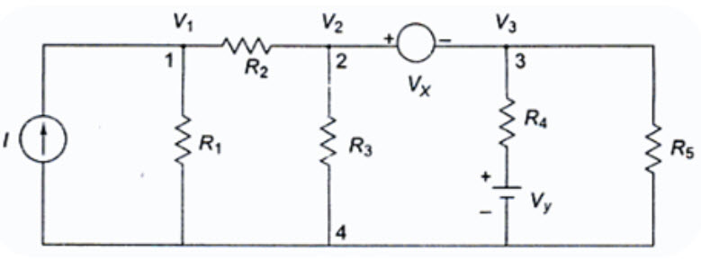
Fig. 7.1

It is clear from Fig. 7.1, that node 4 is the reference node. Applying Kirchhoff’s current law at node 1, we get

\[I={{{V_1}} \over {{R_1}}} + {{{V_1} - {V_2}} \over {{R_2}}}\]

Due to the presence of voltage source V_x in between nodes 2 and 3, it is slightly difficult to find out the current.  The supernode technique can be conveniently applied in this case.

Accordingly, we can write the combined equation for nodes 2 and 3 as under.

\[{{{V_2} - {V_1}} \over {{R_2}}} + {{{V_2}} \over {{R_3}}} + {{{V_3} - {V_y}} \over {{R_4}}} + {{{V_3}} \over {{R_5}}}=0\]

The other equation is

V₂ – V₃ = V_x

From the above three equations, we can find the three unknown voltages.

7.2. Source Transformation Technique

In solving networks to find solutions one may have to deal with energy source. It has already been discussed in Chapter 1 that basically, energy sources are either voltage sources or current sources.  Sometimes it is necessary to convert a voltage source to a current source and vice-versa.  Any practical voltage source consists of an ideal voltage source in series with an internal resistance.  Similarly, a practical current source consists of an ideal current source in parallel with an internal resistance as shown in Fig. 7.2.  R_v and R_i represent the internal resistance of the voltage source V_s’ and current source I_s’ respectively.

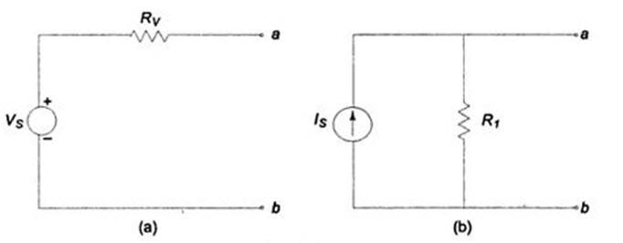Fig. 7.2

Any source, be it a current source or a voltage source, drives current through its load resistance, and the magnitude of the current depend on the value of the load resistance.  Figure 7.3 represents a practical voltage source and a practical current source connected to the same load resistance R_L’

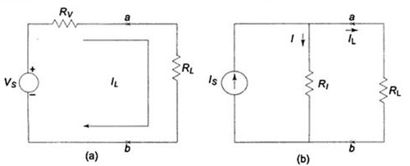
Fig. 7.3

From Fig. 7.3 (a), the load voltage can be calculated by using Kirchhoff’s voltage law as

            V_ab = V_s – I_L R_v

            The open circuit voltage V_OC = V_s

The short circuit current  \[{I_{SC}}\,={{{V_s}} \over {{R_v}}}\]

From Fig. 7.3 (b)

\[{I_L}={I_s} - I={I_s} - {{{V_{ab}}} \over {{R_1}}}\]

The open circuit voltage V_OC = I_s R₁

The short circuit current I_SC = I_S

The above two sources are said to be equal, if they produce equal amounts of current and voltage when they are connected to identical load resistances.  Therefore, by equating the open circuit voltages and short circuit currents of the above two sources we obtain.

            V_OC = I_s R₁ = V_s

\[{I_{SC}}={I_s}={{{V_s}} \over {{R_v}}}\]

It follows that R₁ = R_v = R_s \V_s = I_s R_s

Where R_s is the internal resistance of the voltage or current source.  Therefore, any practical voltage source, having an ideal voltage V_s and internal series resistance R_s can be replaced by a current source I_s = V_s /R_s in parallel with an internal resistance R_s.  The reverse transformation is also possible.  Thus, a practical current source in parallel with an internal resistance R_s can be replaced by a voltage source V_s = I_s R_s in series with an internal resistance R_s.