Electrical Circuits 3(2+1)

LESSON 19. Reactive power and power triangle

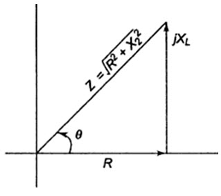
Fig.19.1

\[{P_{av}}`={I_{eff}}\,\,Z\,\left[ {{I_{eff}}\,{R \over Z}} \right]\]

\[=\,\,\,I_{eff}^2\,\,R\,\,watts..................................................\left( {19.4} \right)\]

This gives the average power dissipated in a resistive circuit.If we consider a circuit consisting of a pure inductor, the power in the inductor.

\[{P_r}=i{v_L}..................................................\left( {19.5} \right)\]

\[=iL\,{{di} \over {dt}}\]

Consider \[i={I_m}\,\sin \,(\omega t\, + \,\theta )\]

Then \[{P_r}=I_m^2\,\sin \,\left( {\omega t + \theta } \right)L\omega \,\,\cos \,\,\left( {\omega t + \theta } \right)\]

\[={{I_m^2} \over 2}\,\left( {\omega L} \right)\sin \,\,2\,\,\left( {\omega t + \theta } \right)\]

\[\Pr=I_{eff}^2\left( {\omega L} \right)\,\sin \,2\,\left( {\omega t + \theta } \right)..................................................\left( {19.6} \right)\]

From the above equation, we can say that the average power delivered to the circuit is zero.  This is called reactive power.  It is expressed in volt-amperes reactive (VAR).

\[{P_r}=I_{eff}^2\,{X_L}\;\,VAR..................................................\left( {19.7} \right)\]

From Fig.19.1, we have

\[{X_L}=Z\sin \,\theta ..................................................\left( {19.8} \right)\]

Substituting Eq. 19.8 in Eq. 19.7, we get

\[{P_r}=I_{eff}^2\,Z\,\sin \,\theta \;\]

\[=\left( {{I_{eff}}Z} \right){I_{eff\,}}\sin \,\theta\]

\[=\,{V_{eff}}\,{I_{eff}}\,\,\sin \,\theta \,\,VAR\]

19.2. The Power Triangle

A generalized impedance phase diagram is shown in Fig.19.2.  A phasor relation for power can also be represented by a similar diagram because of the fact that true power P_av and reactive power Pr differ from R and X by a factor I²_eff as shown in Fig. 19.2.

At any resultant in time, P_a is the total power that appears to be transferred between the course and reactive circuit.  Part of the apparent power is true power and part of it is reactive power.

\[{P_a}=I_{eff}^2\,Z\]

The power triangle is shown in Fig19.2

From Fig. 19.3, we can write

\[{P_{true}}={P_a}\cos \,\theta\]

or average power P_av = P_a cos θ

and reactive power P_r = P_a sin θ

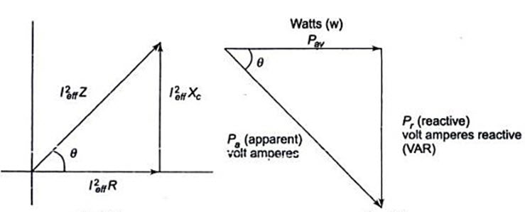
Fig.19.2                                Fig. 19.3