Site pages
Current course
Participants
General
Module 1: Basics of Agricultural Drainage
Module 2: Surface and Subsurface Drainage Systems
Module 3: Subsurface Flow to Drains and Drainage E...
Module 4: Construction of Pipe Drainage Systems
Module 5: Drainage for Salt Control
Module 6: Economics of Drainage
Keywords
12 April - 18 April
19 April - 25 April
26 April - 2 May
Lesson 5 Investigation of Drainage Design Parameters
5.1 Drainage Coefficient and Its Determination
5.1.1 Concept of Drainage Coefficient
The concept of drainage coefficient is used for the design of drainage systems for agricultural lands; it is the key parameter needed for the hydraulic design of drainage systems. In agriculture lands, open ditches or drains are the most commonly used surface drainage structures. The rate at which the open drains should remove water from a drainage area depends on: (i) rainfall, (ii) size of the drainage area, (iii) characteristics of the drainage area, and (iv) nature of the crops grown and the degree of protection required for them from waterlogging.
Drainage coefficient is defined as the amount of surplus water to be removed from the agricultural land in 24 hours so that the plants are not stressed due to surplus water. Alternatively, it is also defined as the depth of water to be removed in 24 hours from the entire drainage area. A commonly used unit of drainage coefficient is cm/day or mm/day. It is also expressed as the flow rate per unit area, i.e., m3/s per km2 or L/s per hectare (Lps/ha). Thus, for a 100 ha agricultural watershed, a drainage coefficient of 1 mm/day would lead to a discharge of 100 ´ 0.116 = 11.6 L/s at the outlet of the watershed (because 1 mm/day = 0.116 Lps/ha).
Drainage coefficient for an agricultural land is decided such that no appreciable damage is caused to the crops to be grown in that land. The intensity of rain and its duration are inversely proportional to the time allowed for removal of water (which depends upon the type of crop). In deciding the drainage coefficient of an area past experience with similar soils, climatic conditions and crops is very useful. For open ditches for small agricultural areas, the value of drainage coefficient ranges from 0.6 to 2.5 cm, and in extreme cases up to 10 cm. Note that the drainage coefficient is an average rate and it does not take into consideration the runoff distribution with time. Conceptually, the drainage coefficient represents a flow rate lower than the peak of the hydrograph (as calculated by the rational formula). The flow rate corresponding to the drainage coefficient should be adjusted in such a way that the volume of water represented by the area of the direct runoff hydrograph above the drainage coefficient is able to flow out of the watershed within a duration during which it is not harmful for the plants.
Example Problem (Murty and Jha, 2009): A watershed of 1500 hectares is discharging through a drain at an average ratio of 2.5 m3/s. Calculate the drainage coefficient. If the drainage coefficient is 3 cm, what would be the discharge through the drain?
Solution:
Drain discharge in 24 hours = 2.5 ´ 60 ´ 60 ´ 24 m3/day.
= 0.0144 m per day = 1.44 cm/day, Ans.
If the drainage coefficient is 3 cm, the rate of flow through the drain (Q) will be:
5.1.2 Determination of Drainage Coefficient
5.1.2.1 Basic Approaches
In watersheds with average land slopes greater than 1 to 2%, the peak runoff rate is calculated by runoff estimation methods such as rational method, SCS triangular hydrograph method and empirical formula. However, in flat areas (land slopes less than 1%), it is essential to consider the time interval for removing a certain volume of excess surface water (surface waterlogging) occurring with a certain probability. The runoff for the design of open ditches is expressed as drainage coefficient.
A design drainage coefficient is obtained by considering the runoff from a design rainfall. A design rainfall may be considered as the rainfall of a given duration with a given recurrence interval. For example, one may determine a drainage coefficient for a 5-year 1-day rainfall. There are two basic approaches for determining drainage coefficient. In the first approach, the estimated runoff from the design rainfall is distributed over time by following a certain calculation procedure. The result is a hydrograph of flow with a peak. Under this approach, design drainage rate can also be estimated by using some empirical relations. The drainage channel capacity is determined to carry the peak flow as obtained from the above analysis. Such a procedure will result in two large dimensions of drainage channel cross-section which is not required and will be expensive. In the second approach, for designing the capacity of a drainage channel, a certain time is assumed as the time within which the excess runoff has to be removed. A safe excess water removal period may be considered as 2 days. This is based on the assumption that if the excess water is removed from the field within 2 days, there may not be any irreversible adverse effect on the plant, and hence on the crop yield. Therefore, it would be appropriate to consider a 2-day rainfall of a desired recurrence interval as the design rainfall, determine the corresponding direct runoff, and divide this by the stipulated period of excess water removal to get the value of design drainage coefficient.
Both the above approaches are indirect estimation of drainage coefficient, and are often used by drainage engineers. However, a more appropriate approach could be to monitor the performance of crops grown under varying drainage conditions or under imposed drainage treatments and work out the most appropriate rate of water removal that leads to an economic design of the drainage systems. An economic drainage system is one which may lead to the desired benefit from drainage (e.g., production at a pre-determined level) at a minimum cost. It is often difficult to quantify the benefits from drainage other than the increase in crop production due to good drainage. Such benefit components are: better trafficability, more field working days, lesser insect-pest attack, and so on. They ultimately help in increasing crop yields.
5.1.2.2 Methods for Determining Drainage Coefficient
The methods commonly used for determining drainage coefficient (i.e., design capacity of open ditches for drainage) are: (i) Cypress Creek formula, (ii) Boston Society formula, and (iii) Simplified Hydrologic Accounting method. These methods are briefly described below.
(1) Cypress Creek Formula
An empirical relationship relating design drainage rate at the outlet of a watershed and the watershed area was developed in the USA based on the data from a large number of watersheds. This relationship is popularly known as the Cypress Creek formula and is considered valid for a mean watershed slope of £0.45%. This relationship was developed based on the fact and observations that the unit drainage rate (discharge per unit area) reduces as the watershed area increases. Accordingly, an equation relating the runoff rate with the watershed area was obtained as follows:
Where, Q = runoff rate (m3/s), A = area of the watershed or agricultural land (km2), p = 5/6 (Approximate average value), and C = (0.2098 + 0.0074Y), where Y is the direct runoff volume (mm) estimated by the CN method.
This formula is entirely empirical and has been derived upon a large number of observations carried out in the USA. The value of Q is not the same as peak discharge, and it may so happen that its value will be much less than the peak discharge as certain amount of flooding is allowed before the water is drained.
Since the value of p in Eqn. (5.1) is less than 1, the rate of increase in the estimated design discharge will not be proportional to the increase in the drainage (watershed) area. This equation makes use of the CN-estimated runoff which is reflected in the coefficient ‘C’. The value of p as 5/6 was standarised based on the analysis of the runoff data from the watershed of different sizes.
Assuming that Eqn. (5.1) is applicable to the climatic conditions of India, a few average values of C in the equation for estimating a 5-year return period (recurrence interval) Q are given in Table 5.1. For obtaining the design runoff for a 2-year return period, the values of Q, calculated using Eqn. (5.1) for the C values listed in Table 5.1, are to be multiplied by a factor varying between 0.79 and 0.84 for different regions of India. These values have been obtained from the drainage area-design discharge curves for different regions of India and for three major groups of crops as developed by Gupta et al. (1971). The design discharge was calculated based on the volume of runoff estimated by the CN method for a constant Ia versus S relation of Ia = 0.2S. Eqn. (5.1) is further used to proportion the design discharge based on the size of the contributing segments of a watershed at a given junction of two drains. Based on the field studies, it has been found that the Cypress Creek formula considerably over estimates the drainage coefficient for watershed areas up to about 100 km2.
Table 5.1. Average values of the coefficient (C) appearing in the Cypress Creek formula (Gupta et al., 1971)
|
Sl. No. |
Region |
Values of ‘C’ for Different Crops |
||
|
Vegetable Crops |
Grain Crops |
Rice |
||
|
1 |
Punjab and Haryana Alluvial Soils |
1.414 |
0.354 |
0.071 |
|
2 |
Indo-Gangetic Alluvial Soil (North) |
3.084 |
1.050 |
0.421 |
|
3 |
Indo-Gangetic Alluvial Soil (South) |
2.375 |
0.668 |
0.260 |
|
4 |
Indo-Gangetic Alluvial Soil (Central) |
2.820 |
0.816 |
0.185 |
|
5 |
Black Soil (sub-humid) |
4.454 |
1.113 |
0.890 |
|
6 |
Black Soil (arid and semi-arid) |
2.970 |
0.519 |
0.372 |
|
7 |
Eastern Red Soils |
3.396 |
1.050 |
0.734 |
|
8 |
Southern Red Soils |
2.262 |
0.565 |
0.356 |
|
9 |
Assam Valley |
2.970 |
0.927 |
0.446 |
(2) Boston Society Formula
Peak discharge for the design of surface drains suggested by the Boston Society of Civil Engineers is given as:
![]()
Where, Q = peak discharge in cusec (ft3/s), C = coefficient, and A = peak catchment area in square miles. Uppal and Sehgal (1965) reported the values of C (Table 5.2) appearing in Eqn. (5.2). These proposed values are mainly applicable for the catchments in different parts of Punjab and Haryana states.
Table 5.2. Values of coefficient (C) appearing in the Boston Society formula (Uppal and Sehgal, 1965)
|
Sl. No. |
Catchment Area (Square miles) |
Values of ‘C’ for Different Rainfalls |
||
|
For Rainfall less than 20 inches |
For Rainfall between 20 and 30 inches |
For Rainfall between 30 and 40 inches |
||
|
1 |
0-25 |
20 |
50 |
100 |
|
2 |
25-100 |
50 |
100 |
250 |
|
3 |
100-250 |
100 |
200 |
450 |
|
4 |
Above 250 |
200 |
400 |
600 |
Note: For rainfall above 40 inches, a value of C of 2500 irrespective of the catchment area is suggested.
In order to economise the construction of drainage systems, the surface drains are sometimes designed for a discharge ranging from 1/4 to 1/12 of the calculated peak discharge (Dhruvanaryana, 1980). The practical consideration is to remove the excess water due to heavy storms from the cropped fields within seven days. The drainage systems on Sarda Canal Project in Uttar Pradesh, India were designed for a capacity of 0.11 m3/s per km2 of the catchment, whereas the drainage systems in Punjab were designed for a capacity of only 0.04 m3/s per km2 of the catchment.
(3) Simplified Hydrologic Accounting Method
The method given by Raadsma and Schulze (1974) consists of analyzing the rainfall data and estimating the number of hours required to remove the excess water using the information about crop tolerance.
The rainfall data are analyzed for duration-frequency. As drainage is planned taking crop into consideration, the rainfall duration-frequency for a particular crop season is considered. The rainfall excess is calculated and allowance is made for channel storage. Knowing the drainage coefficient, i.e., the depth of water to be removed in 24 hours, the capacity of the drainage system required can be obtained. The example presented below illustrates the application of this method using hypothetical data (Murty and Jha, 2009).
Table 5.3. Example rainfall data for drainage design (Source: Murty and Jha, 2009)
|
Sl. No. |
Return Period |
Type of Rainfall |
Duration of Rainfall |
|||
|
90 min |
24 h |
48 h |
72 h |
|||
|
1 |
1 ´ 2 year |
Annual |
40 |
65 |
95 |
105 |
|
Seasonal |
30 |
55 |
78 |
93 |
||
|
Excess (1) |
16 |
30 |
52 |
66 |
||
|
Excess (2) |
6 |
20 |
42 |
56 |
||
|
2 |
1 ´ 5 year |
Annual |
50 |
86 |
120 |
140 |
|
Seasonal |
40 |
72 |
85 |
120 |
||
|
Excess (1) |
25 |
48 |
58 |
90 |
||
|
Excess (2) |
15 |
38 |
48 |
80 |
||
|
3 |
1 ´ 10 year |
Annual |
60 |
105 |
140 |
165 |
|
Seasonal |
50 |
85 |
120 |
150 |
||
|
Excess (1) |
35 |
55 |
90 |
120 |
||
|
Excess (2) |
25 |
45 |
80 |
110 |
||
In this example, storage of 10 mm is uniformly assumed in the surface channels. The information given in Table 5.3 is plotted as shown in Fig. 5.1. In addition, drainage capacities are plotted. These graphs can be used to determine the drainage capacity or for a given drainage capacity, the number of hours required to remove excess surface water. For instance, with a drainage capacity of 30 mm/24 hours, a rainfall excess occurring once in 5 years can be drained in about 40 hours (Fig. 5.1). This method is useful when a single crop is involved and its drainage coefficient is known. However, if more crops are involved, the calculation should be done for individual crops.
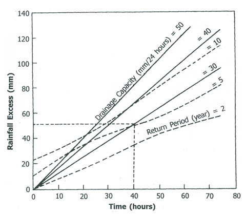
Fig. 5.1. Number of hours required to remove excess surface water.
(Source: Murty and Jha, 2009)
Pai and Hukkeri (1979) recommended that the drains should be designed for 1-day average of 3-day maximum rainfall of 5-year return period with a runoff percentage, calculated after taking into account infiltration rate, evaporation and permissible water storage in the fields or calculated by rainfall-runoff observations. If no field data are available for the area under study, the runoff percentage for different types of soils and for varying intensity of vegetation as given in Table 5.4 can be adopted. The period of disposal of rainfall depends on the type of crops and their growth stages. The values of drainage periods recommended by Pai and Hukkeri (1979) are summarized in Table 5.5.
Table 5.4. Recommended runoff percentage for different soils and vegetation intensities (Source: Murty and Jha, 2009)
|
Sl. No. |
Type of Soil |
Runoff (%) |
|
1 |
Sandy soils |
20 |
|
2 |
Loamy soils (largely cultivated) |
30 |
|
3 |
Loamy soils (lightly covered by crops) |
40 |
|
4 |
Gardens and cultivated areas |
5 to 25 |
Table 5.5. Recommended drainage periods for selected crops (Source: Pai and Hukkeri, 1979)
|
Sl. No. |
Type of Crop |
Drainage Period |
Remarks |
|
1 |
Paddy and Sugarcane |
7 days |
Panicles in the case of paddy not to get sub-merged and depth of ponding for temporary period not to be more than 0.5 m. |
|
2 |
Pearl Millet and Cotton |
3 days |
3 day rainfall to be drained in 3 days. |
|
3 |
Sorghum and Maize |
2 days |
2 day rainfall to be drained in 2 days. |
|
4 |
Vegetables |
1 day |
24 hour rainfall to be drained in 24 hours. |
5.2 Determination of Hydraulic Conductivity
To determine a representative value of hydraulic conductivity (K), the drainage surveyor must have a theoretical knowledge of the relationships between the kind of drainage system envisaged and the drainage conditions prevailing in the survey area. For example, the surveyor should have some idea about the relationship between effectiveness of drainage and such information as: (i) drain depth and the value of K at this depth, (ii) depth of groundwater flow and the type of aquifer, (iii) variation in hydraulic conductivity with depth, and (iv) the anisotropy of the soil. A variety of laboratory and field methods exist to determine soil hydraulic conductivity, with varying degrees of accuracy. The pros and cons of different methods of hydraulic conductivity determination are succinctly described below.
5.2.1 Methods for Determining Hydraulic Conductivity
The methods for determining hydraulic conductivity (K) of a soil can be classified into two broad groups: (1) correlation methods, and (2) hydraulic methods. Hydraulic methods of K determination can be further divided into two groups: laboratory methods and field methods. An overview of these methods is presented below.
5.2.1.1 Correlation Methods
Correlation methods are based on predetermined relationships between an easily determined soil property (e.g., texture, pore-size distribution, grain-size distribution, etc.) and the hydraulic conductivity (K). A variety of empirical formulae are available which relate K with content of sand, silt and clay; K with grain diameter (mean or effective grain diameter); K with grain-diameter and porosity; K with grain-size distribution; and K with soil series (Oosterbaan and Nijland, 1994; Domenico and Schwartz, 1998), and they can be used in the absence of field or laboratory values of hydraulic conductivity. For example, Smedema and Rycroft (1983) provided a generalized table with ranges of K-values for certain soil textures as shown in Table 5.6. However, such tables should be handled with care. Smedema and Rycroft (1983) warn that: “Soils with identical texture may have quite different K-values due to differences in structure and some heavy clay soils have well-developed structures and much higher K-values than those indicated in the table”.
Table 5.6. Values of K by soil texture (Smedema and Rycroft, 1983)
|
Sl. No. |
Soil Texture |
Range of K (m/day) |
|
1 |
Gravelly coarse sand |
10 – 50 |
|
2 |
Medium sand |
1 – 5 |
|
3 |
Sandy loam, fine sand |
1 – 3 |
|
4 |
Loam, clay loam, clay (well structured) |
0.5 – 2 |
|
5 |
Very fine sandy loam |
0.2 – 0.5 |
|
6 |
Clay loam, clay (poorly structured) |
0.002 – 0.2 |
|
7 |
Dense clay (no cracks, pores) |
<0.002 |
Of the various empirical formulae, the Hazen formula is a simple relationship between the hydraulic conductivity and the effective grain diameter, and it is often used for the estimation of hydraulic conductivity from grain-size distribution data. It is expressed as (Freeze and Cherry, 1979):
K = A × d102 (5.3)
Where, K = hydraulic conductivity, (cm/s); d10 = effective grain diameter, (mm) which is determined from the grain-size distribution curve; and A = constant, which is usually taken as 1.0 (Freeze and Cherry, 1979).
The advantage of the correlation methods is that an estimate of the K value is often simpler and faster than its direct determination. However, the major drawback of these methods is that the empirical relationship may not be accurate in all cases, and hence may be subject to random errors.
5.2.1.2 Hydraulic Methods
Hydraulic methods are based on imposing certain flow conditions in the soil and applying an appropriate formula based on the Darcy’s law and the boundary conditions of the flow. The value of K is calculated from the formula using the values of hydraulic head and discharge observed under the imposed conditions. Hydraulic methods can be classified into two groups: laboratory methods and field (in situ) methods.
The hydraulic laboratory methods are applied to core samples (undisturbed samples) of the soil and saturated hydraulic conductivity can be determined by using constant head method or falling head method; the details about this method can be found in standard textbooks on irrigation or drainage (e.g., Murty and Jha, 2009; Smedema and Rycroft, 1983). Although hydraulic laboratory methods are more laborious than the correlation methods, they are still relatively fast and cheap, and they eliminate the uncertainties involved in relating certain soil properties to the hydraulic conductivity of the soil. However, regarding variability and representativeness, they have similar drawbacks as the correlation methods (Oosterbaan and Nijland, 1994). Owing to the small-size of core samples, one must obtain a large number of core samples for obtaining a representative value of K. Also, if used on a large scale, hydraulic laboratory methods are very laborious and time consuming.
In contrast to the hydraulic laboratory methods, which determine K inside a core with fixed edges, the field or in situ methods usually determine K around a hole made in the soil so that the outer boundary of the soil mass investigated is often not exactly known. The hydraulic field methods can be divided into two groups: small-scale methods and large-scale methods. The small-scale field methods are designed for rapid testing at many locations. They impose simple flow conditions to avoid complexity so that the measurements can be made relatively quick and cheap. The field methods usually represent the K-value of larger soil mass than the laboratory methods, and hence the variability in the results is relatively less, but can often still be considerable. A drawback of the small-scale field methods is that the imposed flow conditions are often not representative of the flow conditions corresponding to the drainage systems to be designed or evaluated. On the other hand, the large-scale field methods are designed to obtain a representative K-value of a large soil mass, whereby the problem of variation is eliminated to a greater extent. These methods are very reliable, but are more expensive and time consuming than the methods mentioned above.
(1) Small-Scale Field Methods
Various small-scale field methods for the determination of hydraulic conductivity are available (Bouwer and Jackson, 1974). The methods fall into two groups: (a) methods used to determine K above the water table (unsaturated zone), which are known as infiltration methods, and (b) the methods used to determine K below the water table (saturated zone/aquifer), which are known as extraction methods. Note that the small-scale in situ methods are not applicable to large depths, and hence their results are not representative for deep aquifers (Oosterbaan and Nijland, 1994). Thus, the results of small-scale methods are more valuable in shallow aquifers than in deep aquifers.
Infiltration Methods: To measure the saturated hydraulic conductivity of a soil (i.e., K above the water table), one has to apply sufficient water to obtain near-saturated (or field-saturated) conditions. These methods are called infiltration methods and use the relationship between the measured infiltration rate and hydraulic head to calculate K. The equation describing this relationship is selected according to the boundary conditions induced (Oosterbaan and Nijland, 1994). The infiltration methods can be divided into steady-state methods and unsteady-state methods. Steady-state methods are based on the continuous application of water in the hole so that the water level is maintained constant, i.e., the infiltration rate becomes constant. An example of a steady-state infiltration method is ‘shallow well pump-in method’ (Bouwer and Jackson, 1974). A modified form of the shallow well pump-in method is the ‘Guelph permeameter method’, which uses a specially developed apparatus and is based on both saturated and unsaturated flow theory (Reynolds and Elrick, 1985). Interested readers are referred to Bouwer and Jackson (1974), Oosterbaan and Nijland (1994), and Reynolds and Elrick (1985) for the detailed methodology of these steady-state infiltration methods.
In contrast, unsteady-state methods are based on observing the rate of fall of the water level below which the infiltration occurs, after the application of water has been stopped. This measurement can start only after sufficient water has been applied to ensure the saturation of a large enough part of the soil around and below the place of measurement. Bouwer and Jackson (1974) present a number of unsteady-state methods, of which the ‘double-tube method’ is commonly used. Another unsteady-state method is called ‘inversed auger-hole method’ (Oosterbaan and Nijland, 1994), wherein an uncased hole is used. The detailed procedures for using these methods can be found in Bouwer and Jackson (1974), and Oosterbaan and Nijland (1994).
In general, the infiltration methods measure K in the vicinity of the infiltration surface. Hence, it is not easy to obtain K values at greater depths in the soil. Depending on the dimensions of the infiltrating surface, the infiltration methods yield either horizontal K values (Kh), vertical K values (Kv), or K values in an intermediate direction (Oosterbaan and Nijland, 1994). The infiltration methods are more often used for specific research purposes than for routine measurements on a large scale.
Extraction Methods: To measure the saturated hydraulic conductivity of a soil below the water table, one has to remove water from the soil (because the soil is saturated), create a sink, and then observe the flow rate of water into the sink together with the hydraulic head induced. These methods are called extraction methods and use the equation fitting to the boundary conditions to calculate K. The most frequently used extraction method for irrigation and drainage purposes is the ‘auger-hole method’, which is based on the principle of unsteady-state flow (Oosterbaan and Nijland, 1994). Another well-known extraction method is ‘piezometer method’ (Bouwer and Jackson, 1974), which is based on the same principle as the auger-hole method, except that a tube is inserted into the hole, thereby leaving a cavity of limited height at the hole bottom.
As the depth of the hole made for water extraction is large compared to its radius, the flow of groundwater to the hole is mainly horizontal, and hence the extraction methods predominantly yield horizontal K (Kh) values. The extraction methods measure K for a larger soil volume (0.1 to 0.3 m3) than the laboratory methods, and therefore the values of K obtained by these methods are more reliable.
(2) Large-Scale Field Methods
Large-scale field methods are designed for determining hydraulic conductivity below the water table (i.e., K of the saturated zone). The methods available for large-scale K determination are of two types (Oosterbaan and Nijland, 1994): (a) the method that uses pumping from wells (known as ‘pumping test’), and (b) the method that uses pumping or gravity flow from horizontal drains (known as ‘parallel drains method’). The pumping test is the standard and most accurate method for determining ‘hydraulic conductivity’ and ‘storage coefficient’ of saturated zones (aquifers). The detailed methodology for determining K by the pumping test can be found in Groundwater Hydrology books such as Todd (1980), Raghunath (2007), or Fetter (2000).
Using the parallel drains method, hydraulic conductivity (K) can be determined from the functioning of drains in experimental fields, pilot areas, or on existing drains (Oosterbaan and Nijland, 1994), and thus this method is very suitable for drainage. This method uses observations on drain discharges and corresponding elevations of the water table in the soil at some distance from the drains. From these observed data, the value of K can be calculated using a drainage formula (either steady-state or unsteady-state formula) appropriate for the conditions under which the drains are functioning. Since random deviations of the observations from the theoretical relationship frequently occur, a statistical confidence analysis is necessary (Oosterbaan and Nijland, 1994). Note that the analysis of functioning of existing drains under unsteady-state conditions offers an additional possibility of determining another important hydraulic parameter namely ‘drainable porosity’ (discussed in the subsequent section).
The advantage of large-scale determination is that the flow paths of the groundwater and the natural irregularities of the K values along these paths are automatically taken into account in the overall K value found by the method. Therefore, it is not necessary to determine the variation in K values from place to place as well as in horizontal and vertical directions, and the overall K value found can be used directly as an input to the drainage formulae (Oosterbaan and Nijland, 1994). A second advantage is that the variation in K values found is considerably less than those found with small-scale field methods.
5.3Concept and Determination of Drainable Porosity
5.3.1 Concept of Drainable Porosity
The concept of ‘drainable porosity’ is applicable for saturated soils and is very important for the analysis of unsteady flow to drains and for estimating groundwater recharge. When a saturated soil is allowed to drain under gravity, some of the water will drain out. The amount of water drained depends on the size of the pores present in the soil. The large-size pores will drain rapidly followed by medium-size pores and the small-size pores drain very slowly. The volume of water drained under gravity by the coarse-textured soils is more than that by the fine-textured soils. This is due to the fact that coarse-textured soils have greater percentage of large-size pores, while fine-textured soils have greater percentage of small and narrow pores.
The term ‘drainable porosity’ is defined as “the volume of water drained by gravity per unit volume of the saturated soil”. It is also called ‘effective porosity’ or ‘specific yield’ or ‘storage coefficient’, especially in groundwater hydrology or hydrogeology. Since the release of water from a saturated soil under gravity is not instantaneous rather a slow process, the drainable porosity is a function of time and water table depth. However, most drain design methods adopt an average and constant value of drainable porosity because of simplicity in design computations.
5.3.2 Determination of Drainable Porosity
Drainable porosity can be measured in the laboratory or in the field. In the laboratory, drainable porosity can be measured using Hanging Water-Column apparatus (Fig. 5.2) which is suitable for a tension range of 0-150 cm. Hanging Water-Column apparatus consists of a glass funnel with a porous plate, a burette, and a flexible transparent tube connecting the glass funnel and the burette.
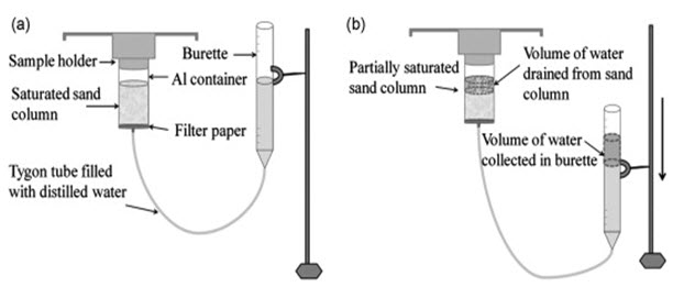
Fig. 5.2. Hanging-Water Column apparatus: (a) Initial saturated sand column; (b) Lowered burette.
(Source: Kang et al., 2012)
Undisturbed soil sample is taken from the field and it is saturated in the laboratory with the help of Hanging Water-Column apparatus (Fig. 5.2a). The saturation may take 24 hours or more depending on the soil type. The water level in the burette is maintained at the same level as the top of the porous plate. Thereafter, the burette is lowered by a certain distance (usually in steps of 10 cm), which imparts a suction to the saturated soil sample, and hence water starts draining slowly (Fig. 5.2b). The drained water raises the water level in the burette. At a given suction, this rise in water level is adjusted by readjusting the burette height such that the originally applied suction is closely maintained. When there is no further rise in water level in the burette, the elevation difference between the top of the porous plate and the water level in the burette are noted down, which gives the value of average suction applied to the soil sample. The difference between the initial and the final burette readings gives the volume of water drained from the soil sample due to the applied suction. This process is repeated by lowering the burette in steps of 10 cm initially and more lately until the desired suction (corresponding to the maximum possible depth of the subsurface drain or any other criteria) is obtained. Generally, applying a suction of greater than 2 m is not required for drainage related studies. Based on the cumulative volume of water drained, drainable porosity is calculated by dividing the volume of water drained with the volume of the soil sample. Note that the Hanging Water-Column apparatus facilitates the determination of drainable porosity of a soil at small and closer suction values that usually occur under subsurface drainage.
Moreover, the drainable porosity can be measured in the field by observing the subsurface drain discharge and the water table recession over a period when the evaporation is insignificant. Generally, the field method provides more accurate values of drainable porosity than the laboratory method.
In practice, drainable porosity is considered as a static soil hydraulic parameter, which represents the average change in the water content of the soil profile when the level of water table changes with a discrete step. Its value depends on soil texture and structure, and the depth of water table. To calculate a practical mean value of the drainable porosity for an area, it should be calculated for the major soil series and for several depths of the water table. If the water retention characteristic of the soil is known and if the pressure-head profile is known for two different levels of water table, the drainable porosity (m) can be calculated from the following equation:
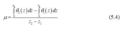
Where, z1 = water table depth (m) for Stage 1 (say at t = t1), z2 = water table depth (m) for Stage 2 (say at t = t2), q1 (z) = soil-water content as a function of soil depth for the water-table position at t1, and q2 (z) = soil-water content as a function of soil depth for the water-table position at t2.
Thus, ‘drainable porosity’ can also be defined as “the ratio of the change in soil-water content in the soil profile above the water table to the corresponding rise/fall of the water table in the absence of evaporation”.
The above definition of drainable porosity is illustrated in Fig. 5.3A. In this figure, the soil-water content of a silty clay soil is shown by the line A-B for a water table depth of 0.50 m, and by the line C-D for a water table depth of 1.20 m. The drainable porosity in this case is represented by the enclosed area ABCD (representing the change in soil-water content) divided by the change in water table depth AD. That is,
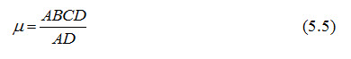
Usually, the drainable pore space is calculated for equilibrium conditions between soil-water content and water table depth. Note that the drainable porosity for a given soil is not a constant for the entire soil profile; rather it depends on the depth of the water table. Generally, drainable porosity increases with increasing water table depths. The capillary reach in which equilibrium conditions exist is only active where the soil surface is nearby and when soil water is occasionally removed by evaporation. For a depth greater than a certain critical value (which depends on the soil type), the drainable porosity can be approximated by the difference in soil moisture (q) between field capacity and saturation.
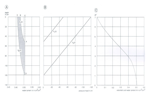
Fig. 5.3. (A) Soil-water profiles for equilibrium conditions with the water table at 0.50 m [q1(z)] and at 1.20 m [q2(z)].
The area enclosed by q1(z), q2(z), the soil surface, and AD represents drainable porosity;
(B) Equilibrium pressure-head profiles for water tables at 0.50 and 1.20 m;
(C) Soil-water retention curve for a silty clay soil. (Source: Kabat and Beekma, 1994)
Typical values of drainable porosity (m) for field soils vary from 2 to 10% (Smedema and Rycroft, 1983). A m-value of 5% indicates that the water table falls or rises by 10 cm for each 5 mm of water extracted from or added to the groundwater, respectively. If the values of m are small, the response of water table to the extraction or addition of water is large, and the reverse is true for large m-values. Table 5.7 summarizes representative values of drainable porosity for salient soils.
Table 5.7. Drainable porosity for different soils (Smedema and Rycroft, 1983)
|
Sl. No. |
Soil Type |
Drainable Porosity (%) |
|
1 |
Dense Clay |
1 to 2 |
|
2 |
Well Structured Loams, Clay Loams and Clays |
4 to 8 |
|
3 |
Fine Sand |
15 to 20 |
|
4 |
Coarse Sand |
25 to 35 |
Example Problem on Drainable Porosity (Bhattacharya and Michael, 2003): In a subsurface drainage network, 10 lateral drains laid at a spacing of 40 m and each 150 m long, join a collector drain. The average discharge at the outlet of the collector drain was 10 L/s when the water table dropped from ground surface to 40 cm below the ground surface in 3 days. Find the average drainable porosity of the soil.
Solution:
Total area drained = 10 ´ 150 ´ 40 = 60,000 m2
Volume of soil drained = 60,000 ´ 0.4 = 24,000 m3
Volume of water drained in 3 days = 10 ´ 3600 ´ 24 ´ 3/1000 = 2592 m3.
There for, Drainable Porosity = 2592 ÷ 24000 = 0.108 or 10.8%, Ans.
The above calculated value of drainable porosity is the average of the top 40 cm soil layer and also an average over the time period of 3 days. As the water table is gradually declining, the discharge rate will also gradually decline. If the information on the discharge for shorter durations and the corresponding water table decline were available, the drainable porosity calculated for the shorter duration would have been different. Furthermore, the computed value of drainable porosity is also approximate as the entire depth of 40 cm of the soil has been assumed to have experienced a uniform water table decline of 40 cm. However, in a subsurface drained field, the water table is curved between the adjacent parallel drains. Therefore, the drained soil volume is not uniform throughout the drained field.
References
Bhattacharya, A.K. and Michael, A.M. (2003). Land Drainage: Principles, Methods and Applications. Konark Publishers Pvt. Ltd., New Delhi, India.
Bouwer, H., and Jackson, R.D. (1974). Determining Soil Properties. In: J. van Schilfgaarde (editor), Drainage for Agriculture, Agronomy Monograph 17, American Society of Agronomy, Madison, pp. 611-672.
Dhruvanaryana, V.V. (1980). Reclaiming Alkali Soils: Engineering Aspect. Bulletin No. 6, Central Soil Salinity Research Institute, Karnal, India.
Domenico, P.A. and Schwartz, F.W. (1998). Physical and Chemical Hydrogeology. 2nd Edition, John Wiley & Sons, New York.
Fetter, C.W. (2000). Applied Hydrogeology. 4th Edition. Prentice Hall, NJ.
Freeze, R.A. and Cherry, J.A. (1979). Groundwater. Prentice-Hall Inc., Englewood Cliffs, New Jersey.
Gupta, S.K., Tejwani, K.J. and Ram Babu. (1971). Drainage coefficient for surface drainage of agricultural land for different parts of the country. Journal of Irrigation and Power, January-1971 issue, pp. 53-60.
Kabat, P. and Beekma, J. (1994). Water in the Unsaturated Zone. In: H.P.Ritzema (Editor-in-Chief), Drainage Principles and Applications, International Institute for Land Reclamation and Improvement (ILRI), ILRI Publication 16, Wageningen, The Netherlands, pp. 383-434.
Kang, M., Bilheux, H.Z., Voisin, S., Cheng, C.L., Perfect, E., Horita, J. and Warren, J.M. (2012). Water Calibration Measurements for Neutron Radiography: Application to Water Content Quantification in Porous Media. Elsevier, pp. 24-31.
Murty, V.V.N. and Jha, M.K. (2009). Land and Water Management Engineering. Fifth Edition, Kalyani Publishers, Ludhiana, India, pp. 374-387.
Oosterbaan, R.J. and Nijland, H.J. (1994). Determining the Saturated Hydraulic Conductivity. In: H.P.Ritzema (Editor-in-Chief), Drainage Principles and Applications, International Institute for Land Reclamation and Improvement (ILRI), ILRI Publication 16, Wageningen, The Netherlands, pp. 435-476.
Pai, A.A. and Hukkeri, S.B. (1979). Manual on Irrigation Water Management. Department of Agriculture, Krishi Bhavan, New Delhi, India.
Raadsma, S. and Schulze, F.E. (1974). Surface Field Drainage Systems. In: Drainage Principles and Applications, Vol. IV, International Institute for Land Reclamation and Improvement, Wageningen, The Netherlands.
Raghunath, H.M. (2007). Ground Water. Third Edition, New Age International Publishers, New Delhi.
Reynolds, W.D. and Elrick, D.E. (1985). In-situ measurement of field saturated hydraulic conductivity, sorptivity, and the a-parameter using the Guelph Permeameter. Soil Science, 140(4): 292-302.
Smedema, L.K. and Rycroft, D.W. (1983). Land Drainage. Batsford Academic and Education Ltd., London.
Todd, D.K. (1980). Groundwater Hydrology. John Wiley & Sons, New York.
Uppal, H.L. and Sehgal, S.R. (1965). Drainage Requirements of the Punjab State. International Commission on Irrigation and Drainage (ICID), Bulletin 23-31, New Delhi, India.
Suggested Readings
Murty, V.V.N. and Jha, M.K. (2011). Land and Water Management Engineering. Sixth Edition, Kalyani Publishers, Ludhiana, India.
Bhattacharya, A.K. and Michael, A.M. (2003). Land Drainage: Principles, Methods and Applications. Konark Publishers Pvt. Ltd., New Delhi, India.
Ritzema (Editor-in-Chief) (1994). Drainage Principles and Applications. International Institute for Land Reclamation and Improvement (ILRI), ILRI Publication 16, Wageningen, The Netherlands.
Smedema, L.K. and Rycroft, D.W. (1983). Land Drainage. Batsford Academic and Education Ltd., London.
Last modified: Monday, 16 September 2013, 6:12 AM