Ground Water, Wells and Pumps

Lesson 22 Introduction to Groundwater Modeling

In this lesson, fundamentals of modeling with a focus on groundwater modeling are presented. Emphasis is given on understanding the basic concepts of groundwater modeling and its proper applications. Interested readers are referred to Wang and Anderson (1982), Bear and Verruijt (1987), Istok (1989), Anderson and Woessner (1992), Spitz and Moreno (1996), Zheng and Bennett (2002), Rushton (2003), and Bear and Cheng (2010) for the details on the theory and practice of groundwater flow and contaminant transport modeling. 

22.2 What is a Model?

 The term ‘model’ can be defined as “a representation of reality that attempts to explain the behavior of some aspect of it and is always less complex than the real system it represents”. 

Simply put, “A model is a tool or device designed to represent a simplified version of reality (actual/natural systems)”. 

Similarly, we can define hydrologic models and groundwater models. “Hydrologic model is a tool designed to represent a simplified version of real hydrologic systems”. On the same footing, “groundwater model is a tool designed to represent a simplified version of real groundwater systems”.   

Thus, a model is a representation of a portion of the natural or human-constructed world and can reproduce some but not all of its characteristics. It is always simpler than the prototype/natural system and can reproduce some but not all of its characteristics.

 

22.3 Why Modeling?

There are two major technical reasons why we need modeling: (a) natural systems (hydrologic, hydraulic, groundwater, etc.) are very complex and highly dynamic in nature, and hence our current knowledge about these systems is limited; and (b) there are limitations of current measurement techniques, i.e., limited availability of spatially and temporally distributed hydrologic, climatologic, geologic, pedologic, and land-use/land cover data. 

Since we are not able to measure everything we would like to know about hydrologic or hydrogeologic systems, we need a means of extrapolating from available measurements in both space and time, particularly to un-gauged catchments (where data are not available) and into the future (where measurements are not possible) in order to assess the impacts of future hydrological changes. Models provide a means of quantitative extrapolation or prediction, which is finally helpful in decision-making. They can also help guide data-collection activities. Thus, models can be broadly used as one of the following tools (Anderson and Woessner, 1992):

(1) Predictive Tool: Models are used as predictive tools when the objective of hydrologic or groundwater modeling is to predict the impacts of a proposed action on existing hydrologic or hydrogeologic conditions.

(2) Interpretive Tool: Models are used as interpretive or research tools when the objective of modeling is to study system dynamics and understand flow and transport processes. Thus, interpretive modeling helps gain insight into the controlling parameters in a site-specific setting or helps assemble and organize field data and formulate ideas about system dynamics.

(3) Generic Tool: Models can also be used to study processes (e.g., flow or transport processes) in a hypothetical hydrologic or hydrogeologic system, which are called generic applications. Generic models are used to develop management standards and guidelines for a given region or as a screening tool to identify regions suitable or unsuitable for some proposed action. Note that ‘predictive modeling’ essentially requires calibration, whereas ‘interpretive modeling’ and ‘generic modeling’ do not necessarily require calibration.

 

There remains a continuing need for hydrologic, hydraulic, and hydrogeologic modeling to solve practical problems concerning water resources assessment, impacts of climate and anthropogenic activities on water quality and quantity, contamination incidents and mitigation, licensing of groundwater abstractions, flood forecasting and protection, design of water resources systems, and so on. In a nutshell, hydrologic/hydrogeologic models are developed either to guide the formulation of water resource management strategies (including the design of structures) or as tools for scientific research. Virtually, all applications of hydrology/hydrogeology to practical water-resource problems involve the use of models. The importance and the application domain of modeling have expanded to such an extent that modeling is taught as a separate subject in major fields of water resources engineering (e.g., surface hydrology, subsurface hydrology, hydraulics, and environmental engineering), especially in developed nations.

 

22.4 Classification of Hydrologic/Hydrogeologic Models            

A variety of models exist in the fields of hydrology and hydrogeology, and they can be classified based on certain criteria. The classification of various types of models used in hydrology and hydrogeology is shown in Fig. 22.1 based on two commonly used criteria. Hydrologic and hydrogeologic models in general can be classified into two broad groups: (a) material models, and (b) mathematical models (Fig. 22.1a). These two major groups of the hydrologic and hydrogeologic models are briefly described below.

  

   

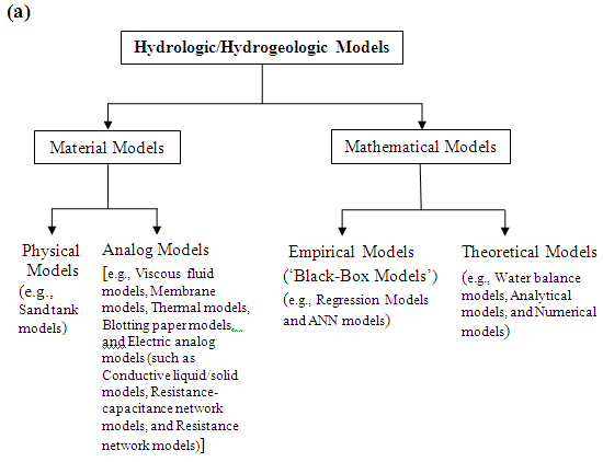
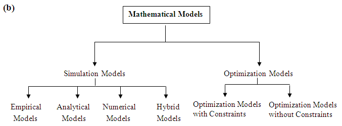
Fig. 22.1. Major classes of hydrologic/hydrogeologic models.

 

22.4.1 Material Models

Material models can be either ‘physical models’ or ‘analog models’. A physical model is a tangible constructed representation of a portion of the natural world (i.e., scaled-down versions of a real system). A miniature, scaled version of a particular watershed and channel and a scaled sand tank model are the examples of physical models. Physical models have been important means to understanding the problems of hydraulics and fluid mechanics, and they are

 

On the other hand, analog models use substances other than (but analogous to) those in a real system. They use observations of one process to simulate a physically analogous natural process. An example of an analog model is an electric analog model in which the flow of electricity represents the flow of water. In the past, a variety of analog models have been used successfully in simulating groundwater flow under various boundary conditions (e.g., Todd, 1980). Other examples of analog models are given in Fig. 22.1(a).

 

22.4.2 Mathematical Models

A mathematical model is a set of mathematical expressions and logical statements combined in order to simulate a natural system. It uses a governing equation thought to represent the physical processes that occur in the system, together with the equations that describe heads or flows along the model boundaries (i.e., ‘boundary conditions’). For time-dependent problems, an equation describing the initial distribution of heads in the system is also required (called ‘initial conditions’). Mathematical models range from a simple linear regression equation to highly complex partial differential equations. 

Mathematical models can be solved analytically using calculus (possible for a limited number of cases), which are known as ‘analytical models’, or they can be solved numerically using numerical techniques (possible for simple as well as complex cases), which are known as ‘numerical models’. Analytical models may or may not involve a computer, but the use of computer is necessary for solving numerical models. The set of commands used to solve a mathematical model on a computer is called ‘computer program’, ‘computer code’, or simply ‘code’. 

As the availability of more powerful computers, modeling techniques and computer software packages has rapidly increased over the past few years, the use of both physical and analog models in hydrology and hydrogeology has been largely replaced by that of computer-implemented mathematical models, which are usually cheaper and much more flexible. 

Mathematical models can also be classified as ‘empirical models’ or ‘theoretical models’ (Fig. 22.1). Empirical models are based on input-output relationships and do not necessarily simulate the actual processes involved. Such models rely on observed input and output data, and simply relate the output to a given set of inputs through a structure which may be fully statistical or partly mathematical. Therefore, empirical models are also known as ‘black-box models’ and they do not help in the physical understanding of processes involved. Examples of empirical models are ‘regression models’ and ‘artificial neural network (ANN) models’. 

In contrast, theoretical models rely on physical laws and theoretical principles. It is assumed that the hydrologic functions or relationships in a system are well understood and can be mathematically approximated directly from system characteristics. Thus, theoretical models use equations derived from basic physics (e.g., conservation of mass, conservation of energy, conservation of momentum, force balance, diffusion, etc.) to simulate flow, transport and storage. Examples are: ‘water balance models’, ‘analytical models’ and ‘numerical models’. Theoretical models are called ‘white-box’ models or ‘grey-box’ models depending on whether model parameters and spatially-varying inputs are considered spatially distributed (white-box models) or lumped (grey-box models) for the model area (basin or sub-basin). Grey-box models are also known as ‘lumped or conceptual models’, whereas white-box models are also known as ‘physically based or process-based models’.  

 

22.5 Elements of Groundwater Modeling

22.5.1 Design and Development of Groundwater Models           

22.5.1.1 Phases of Groundwater Model Development

Mathematical models incorporate the descrip­tions of key processes that determine a system's behavior with varying degrees of sophistication. Hillel (1987) suggests four principles which should guide model development: parsimony, mod­esty, accuracy, and testability. The main phases of numerical groundwater-model development are:

• Compiling and analyzing field data
• Understanding the natural groundwater system
• Conceptualizing the groundwater system
• Selecting a suitable numerical method or code
• Calibrating and verifying/validating the numerical model
• Predicting or simulating future scenarios
• Presenting model results and their analysis

 

In designing and developing a numerical groundwater flow or contaminant (solute) transport model, the first step is data collection and analysis followed by understanding the flow and/or transport processes in a natural groundwater system. The next step is to develop a conceptual model consisting of a description of the physical, chemical and biological processes which are thought to be governing the behavior of the system being modeled (Istok, 1989). A conceptual model is a pictorial representation of the groundwater flow and transport system, frequently in the form of a block diagram or a cross section (Anderson and Woessner, 1992). The nature of the conceptual model determines the dimensions (1-D, 2-D or 3-D) of the numerical model and the design of the grid. The subsequent step is to translate the conceptual model (i.e., our understanding of physical, chemical and biological processes occurring in a real groundwater system) into mathematical terms or a mathematical model (i.e., a set of partial differential equations and an associated set of auxiliary boundary conditions). The resulting groundwater model is only as good as the conceptual understanding of the processes being modeled. Finally, solutions of the governing equations subject to a set of boundary conditions can be obtained by using analytical or numerical methods. For most practical problems, it is not possible to solve the mathematical models analytically because of aquifer heterogeneity and irregular shapes of basin boundaries. Therefore, most groundwater flow and transport simulation models applied in practice are based on the numerical approach. The commonly used numerical methods for solving the partial differential equations of flow and solute transport are: (i) finite difference method (FDM), (ii) finite element method (FEM), (iii) method of characteristics (MOC), and (iv) boundary element method (BEM), among others. However, the FDM and FEM are very popular in subsurface hydrology (e.g., Spitz and Moreno, 1996; Anderson and Woessner, 1992; Wang and Anderson, 1982; Bear and Verruijt, 1987; Istok, 1989).  

 

It should be noted that numerical models are essential for analyzing subsurface flow and contamination problems in a groundwater basin because they are designed to incorporate the spatial variability within a groundwater system as well as spatial and temporal variations in hydrologic parameters that an analytical model cannot incorporate. Numerical solutions are also more flexible and useful than analytical solutions owing to the fact that the user can approximate complex geometries and combinations of recharge and pumping wells by judicious arrangement of grids as well as can easily handle complex boundary conditions. Theoretically, numerical models impose no restrictions on the boundary type, initial conditions, characteristics of the groundwater system, or the characteristics of the solute/contaminant to be investigated.  At present, the use of numerical models is the state-of-the-art in practice for groundwater modeling. In numerical models, the physical layout of the area/basin to be modeled is replaced with a discretized model domain called ‘grid’ which consists of several cells/blocks (if the numerical method used is FDM) or elements (if the numerical method used is FEM). Thus, numerical models basically represent an assembly of many single-cell or single-element models. After developing a numerical model for a given study area (groundwater basin or river basin), it is calibrated and verified (validated) against the observed historical data of hydraulic head or concentration. Once the numerical model is calibrated and verified satisfactorily, various future management scenarios for the study area can be generated without much effort. Finally, model results are analyzed and conclusions/recommendations are made for the problem under investigation. Numerical models can solve both simple and complex problems.

 

22.5.1.2 Modeling Protocol

The above-mentioned phases of model development have been elaborated to formulate a step-by-step procedure for performing numerical modeling. This standard procedure of modeling is known as modeling protocol and is illustrated in Fig. 22.2. Some of the steps of the modeling protocol are described in the subsequent sub-sections, and the complete description of the modeling protocol could be found in Anderson and Woessner (1992).    

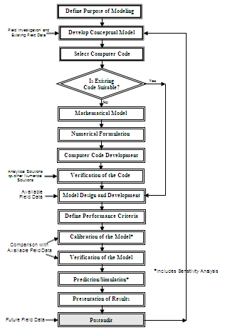
Fig. 22.2. Protocol for model development and application.

(Modified from Anderson and Woessner, 1992)

 

22.5.2 Numerical Solution of Governing Equation           

In order to solve a governing groundwater flow or transport equation (i.e., to compute hydraulic head or solute concentration as a function of x, y, z and t), we need to know aquifer parameters, groundwater sources/sinks as well as the boundary and initial conditions. Thus, the following information is essential to fully define and solve a transient, subsurface flow or transport problem:

(i) The governing equation that applies within the domain (convert physical problem into a mathematical one).

(ii) Size and shape of the region of flow (flow domain).

(iii) Conditions at the boundaries of the flow domain (i.e., boundary conditions).

(iv) Initial conditions within the flow region (i.e., initial conditions).

(v) Spatial distribution of aquifer parameters.

(vi) A mathematical method of solution (e.g., FDM, FEM, or MOC).

 

Computer programs are generally used to solve the mathematical equation using initial and boundary conditions. However, initial conditions are not required for steady-state problems. The set of commands used to solve a mathematical model by a computer is known as computer program or computer code. The computer code is generic, and hence it can be considered as a generic model. When a generic model is applied to represent a particular geographic area by specifying a set of boundary and initial conditions, site-specific grid dimensions as well as site-specific parameter values and hydrologic/hydrogeologic stresses, the resulting computer program is known as a site-specific model. Thus, a computer code is written once but a new model (i.e., site-specific model) is designed and developed for each modeling application. These days, generic computer codes are available for the numerical modeling of groundwater flow and transport processes (e.g., MODFLOW, FEFLOW and FEMWATER) which can be used for different groundwater systems (study areas) without modifying the source codes.

 

It is worth mentioning that the computer code cannot set up the problem. If there is an error in setting up the problem (i.e., understanding the natural system or formulation of the conceptual model), the computer code may give the right answer to the wrong problem! Therefore, it is important to ensure that the problem being solved by the computer code is the same as the one that needs to be solved! Further, running the computer program is fairly straightforward provided that there is good documentation (though tedious sometimes). Setting up the problem, preparing the input data and interpreting the model results are more difficult!

 

22.5.3 Boundary Conditions

The term ‘boundary’ means a geometrical configuration of the surface enclosing the model domain. Boundary conditions must be specified for solving a mathematical model. The boundary conditions constrain the problem at hand and make solutions unique. Mathematically, the boundary conditions include the geometry of the boundary and the values of the dependent variable or its derivative normal to the boundary.

 

Generally, boundary conditions encountered in the field of water resources engineering can be of three types: (i) Dirichlet or Constant-Head Boundary Conditions, (ii) Neumann or Constant-Flux Boundary Conditions, and (iii) Cauchy or Mixed Boundary Conditions.

 

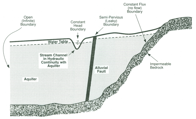
When head or concentration is known for surfaces bounding the model region, it is called Dirichlet boundary condition. Examples of the Dirichlet boundary from groundwater hydrology are: ocean/sea and river/lake in direct hydraulic connection with the aquifer (Fig. 22.3). When flow rate (flux) is known across surfaces bounding the model region, it is called Neumann boundary condition. This type of boundary in groundwater hydrology is used to describe fluxes to surface water bodies, spring flow, and seepage to and from bedrock underlying the aquifer system. A special case of the Neumann boundary condition is when the flux is zero, and then it is also called no-flow boundary condition. Examples of the no-flow boundary from groundwater hydrology are: groundwater divides, streamlines, impermeable faults, and impermeable subsurface layers (Fig. 22.3).

Fig. 22.3. Typical model boundary conditions.

(Source: Roscoe Moss Company, 1990)

 

If some combination of head and flux (i.e., head or water content dependent flux) or of concentration and mass flux (i.e., concentration dependent mass flux) is known for surfaces bounding the model region, it is called Cauchy or head-dependent flux boundary condition. Examples of the Cauchy boundary from groundwater hydrology are: semi-pervious subsurface layers (i.e., leaky confining layers) and semi-permeable or leaky faults (Fig. 22.3).

 

Note that the types of boundaries suitable for a particular field problem require careful consideration. If inconsistent or incomplete boundary conditions are specified, the problem itself will be ill defined!

 

22.5.4 Initial Conditions

Initial conditions are simply the values of the dependent variable specified everywhere inside the boundary (i.e., model domain) at the start of the simulation. Generally, the initial conditions are specified to be a steady-state solution. However, if initial conditions are specified so that transient flow is occurring in the system at the start of simulation, it should be recognized that heads (or concentrations) will change during simulation not only in response to the new pumping stress but also due to the initial conditions.

 

Note that for steady-state problems, only boundary conditions are required to solve a governing equation. However, both boundary and initial conditions are required for transient problems.

 

22.5.5 Calibration and Verification

Calibration of a simulation model is necessary because the real-world hydrogeologic and hydrologic systems are poorly known. Model calibration is defined as “the process in which model parameters are adjusted until the model output matches the field-observed conditions satisfactorily”. For example, in groundwater-flow modeling, calibration is usually accomplished by finding out a set of system parameters (K and S or S_s) and other poorly-known inputs (e.g., recharge and leakance of  streambed or aquitard) that produce simulated values of hydraulic heads and/or fluxes that match the measured/observed values within a specified range of error. Therefore, calibration is sometimes known as ‘parameterization’ or ‘parameter identification’. Model calibration can be performed either by trial-and-error method or by automated technique using an inverse computer code. 

 

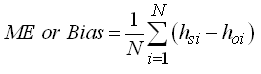
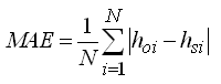
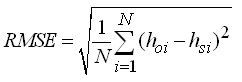
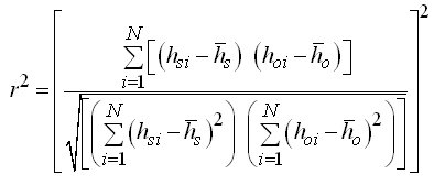
There are no hard and fast rules for deciding a good calibration except that errors between observed and simulated values (hydraulic heads or solute concentrations) should be reasonably small. Several statistical goodness-of-fit criteria have been recommended for evaluating the performance of a model, of which mean error (ME) or bias, mean absolute error (MAE), root mean squared error (RMSE), coefficient of determination (r²),  and Nash-Sutcliffe efficiency (NSE) (also called ‘model efficiency’) are often used. They are mathematically expressed as follows:

 

                           (22.1)

 

                                       (22.2)

 

 

                               (22.3)

 

 

             (22.4)

 

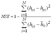                                    (22.5)

 

Where, h_oi = observed groundwater level at the i^th time [L], h_si = simulated (predicted) groundwater level at the i^th time [L], = mean of the observed groundwater levels [L], = mean of the simulated (predicted) groundwater levels [L], and N = total number of the observed data.

 

Besides the statistical goodness-of-fit criteria that facilitate quantitative evaluation, qualitative evaluation is also used for evaluating model performance. Qualitative evaluation involves visual inspection of observed and simulated values in certain graphical ways, for example, simultaneous plots of observed and simulated groundwater-level or concentration hydrographs, their scatter plots, plots of residuals, contour maps, etc.

 

Once the calibration of a model is complete, a verification (or validation) test is usually done so as to ascertain that the model is a valid representation of the hydrogeologic or hydrologic system under study. Model verification is defined as “the process in which the calibrated model is shown to be capable of reproducing a set of field observations independent of that used in model calibration”. Verification results are also assessed using the above-mentioned quantitative and qualitative criteria. During verification, if the observed field conditions are not reproduced with a desired degree of accuracy, the model parameters should be changed to recalibrate the model with a new set of model parameters and the verification run should be repeated. This process eventually results in a calibrated and verified model for a particular study area.

 

22.5.6 Sensitivity Analysis

A well calibrated and verified site-specific model can be reliably used for simulating/predicting future management scenarios as well as for predicting impacts of hydrologic and socio-economic changes. Thereafter, a sensitivity analysis of the developed model is performed. The purpose of a sensitivity analysis is to quantify the effects of uncertainty in the estimates of model parameters on model results. It is usually done by perturbing the values of model parameters (one parameter at a time) by known amounts and measuring the effect of these variations on the model outputs. If a small change in the value of an input parameter produces a large change in the model’s output, the model is said to be sensitive to that parameter and the parameter is said to have a high influence on the model. On the other hand, if a large change in the value of an input parameter produces a small change in the model’s output, the model is said to be insensitive to that parameter and the parameter is said to have a low influence on the model. 

 

Knowledge gained by performing the sensitivity analysis on a model can help to elucidate the way in which the modeled system functions and to identify those parameters of the model whose values need to be specified most accurately during field investigations.

 

22.5.7 Postaudit

As more field data and/or information are collected beyond the model development period (i.e., in the future), it is possible to compare the model predictions against the new set of field data. This process is known as ‘postaudit’ (Fig. 22.2). This may lead to further modifications and refinements (minor or major) of the previously developed ‘site-specific model’ due to significant changes in the system condition with time.

 

22.6 Concluding Remarks

Modeling is an excellent tool to study/understand complex hydrologic and hydrologic systems, and thereby help formulate efficient water management strategies. It facilitates efficient organization, analysis, and synthesis of field data. However, it is important to recognize that modeling is only one component in a comprehensive hydrological or hydrogeological study and not an end in itself. Modeling in conjunction with other tools and techniques can serve as a powerful tool for the planners and decision makers. The key point is that a good modeling methodology, proper knowledge of the system under study, as well as adequate and good-quality data are essential to enhance confidence in modeling analysis and results. Also, establishing the purpose of modeling effort at the outset and establishing realistic expectations can ensure much more effective utilization of modeling.

 

Finally, hydrologists and hydrogeologists (i.e., water resources scientists and engineers) must establish appropriate expectations for the role of modeling in supporting group dynamics and decision-making, and they must understand modeling costs and its actual benefits.

 

 

References

Anderson, M.P. and Woessner, W.W. (1992). Applied Groundwater Modeling: Simulation of Flow and Advective Transport. Academic Press, San Diego.

Bear, J. and Cheng, A.H.-D. (2010). Modeling Groundwater Flow and Contaminant Transport. Springer, New York.

Bear, J. and Verruijt, A. (1987). Modeling Groundwater Flow and Pollution: With Computer Programs for Sample Cases. D. Reidel Publications, Boston.

Bedient, P.B., Rifai, H.S. and Newell, C.J. (1999). Ground Water Contamination: Transport and Remediation. 2^nd Edition, Prentice Hall, N.J.

Fetter, C.W. (1994). Applied Hydrogeology. Third Edition. Prentice Hall, NJ.

Goodchild, M.F. (1993). The State of GIS for Environmental Problem-Solving. In: M.F. Goodchild, B.O. Parks and L.T. Steyart (editors), Environmental Modeling with GIS, Oxford University Press, New York, pp. 8-15.

Hillel, D. (1987). Modeling in Soil Physics: A Critical Review. In Future Developments in Soil Science Research, SSSA, Madison, WI, pp. 35-42.

Istok, J. (1989). Ground Water Modeling by the Finite Element Method. Water Resources Monograph 13, American Geophysical Union (AGU), Washington, D.C.

Jha, M.K. (2011). GIS-based groundwater modeling: An integrated tool for managing groundwater-induced disasters. In: R.H. Laughton (Editor), Aquifers: Formation, Transport and Pollution, Nova Science Publishers, Inc., New York, Chapter 3, pp. 149-190.

Pinder, G.F. (2002). Groundwater Modeling Using Geographical Information Systems. John Wiley & Sons, New York.

Roscoe Moss Company (1990). Handbook of Ground Water Development. John Wiley & Sons, New York.

Rushton, K.R. (2003). Groundwater Hydrology: Conceptual and Computational Models. John Wiley & Sons, Chichester.

Spitz, K. and Moreno, J. (1996). A Practical Guide to Groundwater and Solute Transport Modeling. John Wiley & Sons, New York.

Todd, D.K. (1980). Groundwater Hydrology. John Wiley & Sons, New York.

Wang, H.F. and Anderson, M.P. (1982). Introduction to Groundwater Modeling: Finite Difference and Finite Element Methods. W.H. Freeman and Co., San Francisco.

Zheng, C. and Bennett, G.D. (2002). Applied Contaminant Transport Modeling. John Wiley & Sons, Inc., New York.

 

Suggested Readings

Anderson, M.P. and Woessner, W.W. (1992). Applied Groundwater Modeling: Simulation of Flow and Advective Transport. Academic Press, San Diego.

Wang, H.F. and Anderson, M.P. (1982). Introduction to Groundwater Modeling: Finite Difference and Finite Element Methods. W.H. Freeman and Co., San Francisco.

Bear, J. and Cheng, A.H.-D. (2010). Modeling Groundwater Flow and Contaminant Transport. Springer, New York.

Bear, J. and Verruijt, A. (1987). Modeling Groundwater Flow and Pollution: With Computer Programs for Sample Cases. D. Reidel Publications, Boston.

Spitz, K. and Moreno, J. (1996). A Practical Guide to Groundwater and Solute Transport Modeling. John Wiley & Sons, New York.

Rushton, K.R. (2003). Groundwater Hydrology: Conceptual and Computational Models. John Wiley & Sons, Chichester.