Gulley & Ravine Control Structures

Lesson 20 Models for Predicting Sediment Yield - I

Soil erosion results from a complex interaction of soil-plant-atmospheric forces, often supplemented by anthropogenic forces. Thus, modeling soil erosion requires a multidisciplinary approach among soil scientists, crop scientists, hydrologists, sedimentologists, meteorologists, social scientists and others, notably the engineers who device erosion controls measures and execute them. Models must be able to integrate processes, factors and causes at various spatial and temporal scales. Numerous models of differing prediction capabilities and utilities have been developed. The advent of technological tools such as remote sensing and GIS has significantly enhanced the usefulness of soil erosion models. The coupling of GIS and remote sensing with empirical and process-based soil erosion models has improved their predictive capability. The GIS stores the essential database needed as input or modeling erosion and elaboration of maps of erosion-affected areas. Remote sensing is useful to estimate land cover over large geographic areas, which is a critical input for modeling erosion. Remote sensing and GIS tools also allow the scaling up of modeled data from small plots (e.g., USLE) to large areas. Modeling soil erosion involves integration of complex and variable hydrological processes across large areas to understand the magnitude of soil erosion.

The model should be formulated conceptually, representing it by a flow chart. It is also a good test of the level of scientific understanding of the system and the degree to which the model is to be simplified because of insufficient knowledge. Different types of models for erosion estimation are given in Table 20.1.

Table 20.1 Types of models

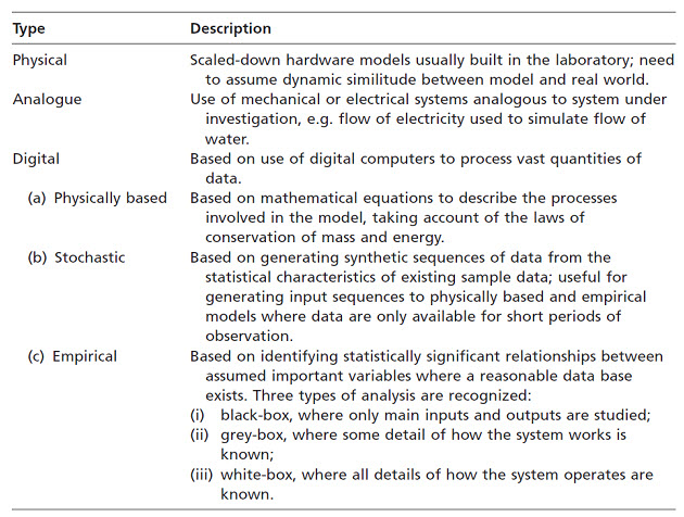
(Source: Morgan, 2005)

A model can be simplified by concentrating on those processes which have the greatest influence over the output and ignoring those which have very little effect. Once the processes operating within the model have been identified, they need to be described mathematically. The methods used can range from simple equations, often expressing a statistical relationship, to complex expressions related to the fundamental physics or mechanics of the process. The former are more common in empirical models, whereas the latter provide the foundation for physically based models.

It is generally recognized that a good model should satisfy the requirements of reliability, universal applicability, easy to use with a minimum of data, comprehensiveness in terms of the factors and erosion processes included and the ability to take account of changes in climate, land use and conservation practice. Unfortunately, many of the ideal characteristics of models conflict with each other. Ease of operation can mean that input data are readily available – for example from an accompanying user’s manual. Such data, however, are at best only guide values and there may be uncertainty in how well they describe actual conditions.

• Model Dimension

(a)Three-Dimensional Model

Flow phenomena in natural rivers are three dimensional, especially those at or near a meander bend, local expansion and contraction, or a hydraulic structure. Sophisticated numerical schemes have been developed to solve truly three-dimensional flow phenomena. Three dimensional models need three-dimensional field data for testing and calibration. The collection of such data is not only costly but also time consuming. Certain assumptions need to be made before a sediment transport formula developed for one-dimensional flows can be applied to a truly three-dimensional model. With the exception of detailed simulation of flow in an estuary area, secondary current, or flow near a hydraulic structure, truly three dimensional models are seldom used, and especially not for long-term simulations.

(b) Two-Dimensional Model

Two-dimensional models can be classified into two-dimensional vertically averaged and two dimensional horizontally averaged models. The former scheme is used where depth-averaged velocity or other hydraulic parameters can adequately describe the variation of hydraulic conditions across a channel. The latter scheme is used where width- or length-averaged hydraulic parameters can adequately describe the variation of hydraulic conditions in the vertical direction. Most two-dimensional sediment transport models are depth-averaged models.

(c) One-Dimensional Model

Most sediment transport models are one-dimensional, especially those used for long-term simulation of a long river reach. One dimensional model requires the least amount of field data for calibration and testing. The numerical solutions are more stable and require the least amount of computer time and capacity. However, one-dimensional models are not suitable for simulating truly two- or three-dimensional local phenomena.

(d) Semi-Two-Dimensional Model

A truly one-dimensional model cannot simulate the lateral variation of hydraulic and sediment conditions at a given river station. Engineers often take advantage of the non-uniform hydraulic and sediment conditions across a channel in their hydraulic design. For example, a water intake structure should be located on the concave side of a meandering bend, where the water is deep and sediment deposition is minimal. There are three types of semi-two dimensional models.

20.2 Empirical Models

Early examples of empirical models include those developed by:

a) Kornev and Kostyakov (1937)

W = a I^0.75 L^0.5 h^1.5                                             (1)

Where,

 W = washout (specific sediment yield); I = slope of ploughed lands;

  L = slope length; h = water return rate; a = correction factor.

b) Glushkov and Polliakov (1946)

a = (S/ 10) I^1/4                                                                 (2)

Where,

 a = erosion coefficient; S = mean annual sediment concentration (g/m³); I = channel slope.

c) Svetitsky (1962)

a_c = P_s /N^1.22                                                                                    (3)

Where,

 a_c = erosion coefficients; P_s= mean annual sediment yield; N = energy characteristic.

Empirical models are developed mostly by relating experimentally generated or records of historical data through the use of coefficients and indices. A theoretical explanation of the empirical relations is generally not feasible.

20.3 SHETRAN Model

SHETRAN is a general, physically-based, spatially-distributed modeling system. It can be used to construct and run models of all or any part of the land phase of the hydrological cycle (including sediment and contaminant transport) for any geographical area. It is physically-based in the sense that the various flow and transport processes are modeled either by finite difference representations of the partial differential equations of mass, momentum and energy conservation, or by empirical equations derived from experimental research. The model parameters have a physical meaning and can be evaluated by measurement. Spatial distributions of basin properties, inputs and responses are represented on a three-dimensional, finite-difference mesh. The channel system is represented along the boundaries of the mesh grid squares as viewed in plan.

20.3.1 SHETRAN Hydrological Component

SHETRAN’s hydrological component consists of subcomponents accounting for evapotranspiration and interception, overland and channel flow, subsurface flow, snowmelt and channel/surface aquifer exchange. The component is continually evolving as new process descriptions and solution schemes are introduced. Integration with the overland flow subcomponent allows overland flow to be generated both by an excess of rainfall over infiltration and by upward saturation of the soil column.

20.3.2 Processes Modeled by the SHETRAN Hydrological Component:

(1) Interception of rainfall on vegetation canopy (Rutter storage model)

(2) Evaporation of intercepted rainfall, ground surface water and channel water; transpiration of water drawn from the root zone (Penman-Monteith equation or the ratio of actual to potential evapotranspiration as a function of soil moisture tension)

(3) Snowpack development and snowmelt (temperature-based or energy budget methods)

(4) One-dimensional flow in the unsaturated zone (Richards equation)

(5) Two-dimensional flow in the saturated zone (Boussinesq equation)

(6) Two-dimensional overland flow; one-dimensional channel flow (Saint Venant equations)

(7) Saturated zone/channel interaction, including an allowance for an unsaturated zone below the channel

(8) Saturated zone/surface water interaction

Flow chart of the SHETRAN model is given below in Fig. 20.1.

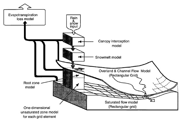
Fig. 20.1. Schematic diagram of the SHETRAN hydrological component. (Source: http://unesdoc.unesco.org/images/0012/001278/127848e.pdf)

20.4 Ephemeral Gully Erosion Model (EGEM)

The EGEM was specifically developed to predict gully formation and erosion based on physical principles of gully bed and side-wall dynamics (Woodward, 1999; Foster and Lane, 1983). Common erosion models such as USLE, RUSLE, and WEPP do not include direct options for predicting gully erosion. The EGEM considers the dynamic processes of concentrated flow responsible for gully incision and head cut development. The EGEM is one of the few process-based models to predict gully erosion.

The EGEM consists of two major components (a) hydrology and (b) erosion. The hydrologic component is estimated using the runoff curve number, drainage area, watershed slope and flow depth, peak runoff discharge, and runoff volume. The erosion component is based on the width and depth of ephemeral channels. The EGEM can predict gully erosion for single storms or seasons or crop stage periods. It assumes that soil erodes to a depth of about 45 cm (e.g., tillage, resistant layer). The width of the gullies is computed using regression equations as:

W_e = 2.66 (Q^0.396) (n^0.387) S^−0.16CS^−0.24

W_u = 179 (Q^0.552)(n^0.556) S^0.199CS^−0.476

Where,

 W_e is equilibrium channel width (m).

 W_u is ultimate channel width (m).

 Q is peak runoff rate (m³ s⁻¹).

 n is Manning’s roughness coefficient.

S is concentrated runoff slope and CS is critical shear stress (Nm⁻²). The detachment rate in gullies is computed similar to that in CREAMS by a modified form of rill erosion equation as follows:

D = KC (1.35t − t_c)

Where,

 D is detachment rate (g⁻² s⁻¹), KC is channel erodibility factor (g s⁻¹ N⁻¹), t is average shear stress of flowing water (Nm⁻²), and t_c is critical shear stress of soil (Nm⁻²)

20.5 EUROSEM Model

EUROSEM (Morgan et al. 1998) is an event-based model designed to compute the sediment transport, erosion and deposition over the land surface throughout a storm, schematic diagram of EUROSEM model is presented in Fig. 20.2. It can be applied to either individual fields or small catchments. Compared with other models, EUROSEM simulates Interrill erosion explicitly, including the transport of water and sediment from Interrill areas to rills, thereby allowing for deposition of material en route. This is considered more realistic than assigning all or a set proportion of the detached material to the rills. A more physically based approach to simulating the effect of vegetation or crop cover is used, taking into account the influence of leaf drainage. Soil conservation measures can be allowed by choosing appropriate values of the soil, micro topography and plant cover parameters so as to describe the conditions associated with each practice. Unlike other models, however, EUROSEM does not describe the eroded sediment in terms of its particle size. The flow chart of the EUROSEM model is given in Fig. 20.2.

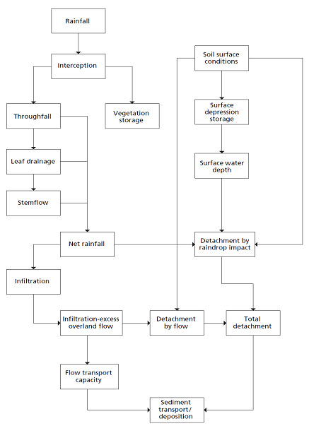
Fig. 20.2. Flow chart for the European Soil Erosion Model (EUROSEM). (Source: European Soil Erosion Model; Morgan et al. 1998;)

EUROSEM has a modular structure with each module being developed in as much detail as the existing level of knowledge permits. This structure will enable continuous improvements to be made in the light of new research. The model deals with:

• The interception of rainfall by the plant cover;

• The volume and kinetic energy of the rainfall reaching the ground surface as direct through fall and leaf drainage;

• The volume of stremflow;

• The volume of surface depression storage;

• The detachment of soil particles by raindrop impact and by runoff;

• Sediment deposition; and

• The transport capacity of the runoff.

20.6 The WEPP (Water Erosion Prediction Project)

WEPP is a process-based continuous simulation erosion model developed by the USDA-ARS that is applicable to both hill-slopes and watersheds, as illustrated in Fig. 20.3. An advantage of WEPP over other existing models such as the popular Universal Soil Loss Equation is that soil loss is estimated spatially at a minimum of 100 points along a profile and deposition of sediment also can be predicted. In other words, soil loss and deposition on a complete continuous hill-slope profile can be calculated, which is important in watershed modeling because it enables enhanced predictions of sediment yields to channels and to the watershed outlet. Additionally, runoff and soil loss are predicted for every rainfall event, allowing detailed temporal analyses and development of probability distributions.

The WEPP watershed model is an extension of the WEPP hillslope model that can be used to estimate watershed runoff and sediment yield. The application of WEPP to a watershed requires that hill slopes be delineated and channels identified. Each hillslope (represented as a rectangle in WEPP) must have a representative length (L), width (W), and slope profile. Hillslopes drain into the top, left side, or right side of a channel, eventually leading to the watershed outlet.

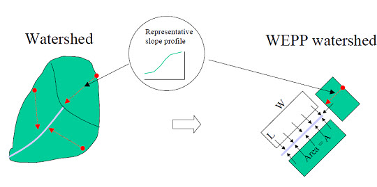
Fig. 20.3. Watershed discretization for WEPP. (Source: http://www.agteca.com/TomThesis/chapter1.pdf)

The erosion model within WEPP applies the continuity equation for sediment transport downslope in the form (Foster & Meyer, 1972):

dQ_s/ dx= D_i+ D_f

Where,

Q_s is the sediment load per unit width per unit time, x is the distance downslope, D_i is the delivery rate of particles detached by Interrill erosion to rill flow and D_f is the rate of detachment or deposition by rill flow. The inter-rill erosion rate (D_i) is given by:

D_i =  K_i I² C_eG_e (R_s /w)

Where,

 K_i is an expression of inter-rill erodibility of the soil, I is the effective rainfall intensity, C_e expresses the effect of the plant canopy, G_e expresses the effect of ground cover, R_s is the spacing of rills and w is the width of the rill computed as a function of the flow discharge. The canopy effect is estimated by:

C_e =1- Fe^-0.34PH

Where,

F is the fraction of the soil protected by the canopy and PH is the canopy height. The ground cover effect is estimated by:

G_e = e^-2.5gi

Where,

gi is the fraction of the Inter-rill surface covered by ground vegetation or crop residue.

The rate of detachment of soil particles by rill flow (D_f) is given by:

D_f = D_c (1- Q_s /T_c )

Where,

D_c is the detachment capacity, Q_s is the sediment load in the flow and T_c is the sediment load at transport capacity. Detachment capacity is expressed as:

D_c = K_r (τ - τ_c )

Where,

K_r is the rill erodibility of the soil, t is the flow shear stress acting on the soil and τ_c is the critical flow shear stress for detachment to occur. The transport capacity of the flow is obtained from:

T_c = k_t τ ^3/2

Where,

k_t is a transport coefficient and τ  is the hydraulic shear acting on the soil. Net deposition occurs if the sediment load is greater than the transport capacity.

20.7 CREAMS Model

CREAM is a field scale model for predicting runoff, erosion, and chemical transport from agricultural management systems. A schematic diagram of the model is shown in Fig. 20.4. It is applicable to field-sized areas. It consists of three major components: hydrology, erosion/sedimentation, and chemistry. CREAMS can operate on individual storms but can also predict long term averages (2-50 years). The objectives of the model were:

• The model must be physically based and not require calibration for each specific application,

• The model must be simple, easily understood with as few parameters as possible and still represent the physical system relatively accurately,

• The model must estimate runoff, percolation, erosion, and dissolved and adsorbed plant nutrients and pesticides and,

• The model must distinguish between management practices.

Based on these objectives, since the management practices were usually on a field basis, the size of a field to represent the scale of the model was needed. A field is defined in the context of the CREAMS model as a management unit having

1) A single land use,

2) Relatively homogeneous soils,

3) Spatially uniform rainfall, and

4) Single management practices, such as conservation tillage or terraces.

Processes and Approach

The hydrologic component consists of two options. When only daily rainfall data are available to the user, the SCS curve number model is used to estimate surface runoff. If hourly or breakpoint rainfall data are available, an infiltration-based model is used to simulate runoff. Water movement through the soil profile is modeled using a simple capacity approach, with flow occurring when a layer exceeds field capacity. The erosion component maintains elements of the USLE, but includes sediment transport capacity for overland flow. The plant nutrient sub-model of CREAMS has a nitrogen component that considers mineralization, nitrification, and denitrification processes. Plant uptake is estimated, and nitrate leached by percolation out of the root zone is calculated. Furthermore, both the nitrogen and phosphorus parts of the nutrient component use enrichment ratios to estimate that portion of the two nutrients transported with sediment. The pesticide component considers foliar interception, degradation, and wash off, as well as adsorption, desorption, and degradation in the soil. Several of the equations developed for the CREAMS model have been used or modified within other models, such as WEPP, SWAT.

Sediment movement down slope obeys continuity of mass:

dq_s/dx = D_L+ D_F

Where,

 q_s is the sediment load per unit width per unit time, x is the distance downslope (m),

D_L is the lateral inflow of sediment (Interrill erosion) (mass per unit area per unit time, i.e. kg m^-2 s^-1), and

D_F is the detachment or deposition of sediment by flow (mass per unit area per unit time, i.e. kg m^-2 s^-1)

The time terms of the full continuity equation drop out under the assumption of quasi-steady state conditions.

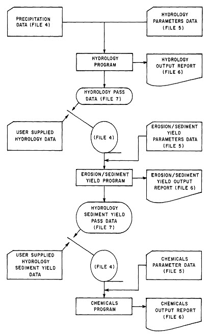
Fig. 20.4. Schematic representation of flow of CREAMS programs. (Source: http://www.tifton.uga.edu/sewrl/Gleams/creams3.pdf)