Remote Sensing & GIS Applications

Lesson- 28 GPS Application

28.1.1. Noise Errors

Noise errors are the combined effect of PRN code noise (around 1 meter) and noise within the receiver noise (around 1 meter).Noise and bias errors combine, resulting in typical ranging errors of around fifteen meters for each satellite used in the position solution. (Dana, 1997)

28.1.2. Bias Errors

Bias errors result from Selective Availability and other factors. Selective Availability (SA) is the intentional degradation of the SPS signals by a time varying bias. It is controlled by the DOD to limit accuracy for non-U. S. military and government users. (Dana, 1997)

Other Bias Error sources are discussed in the later part of the chapter.

28.1.3. Blunders

Blunders can result in errors of hundreds of kilometers. Control segment mistakes due to computer or human error can cause errors from one meter to hundreds of kilometers. User mistakes, including incorrect geodetic datum selection, can cause errors from 1 to hundreds of meters. Receiver errors from software or hardware failures can cause blunder errors of any size. (Dana, 1997)

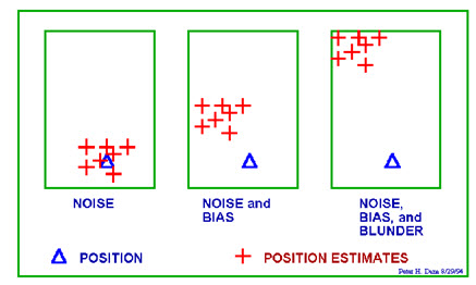
Fig. 28.1. Showing the three types of errors. (Source: Dana, 1997). http://www.ncgia.ucsb.edu/giscc/units/u017/u017.html, posted August 28, 1997.

The analysis of errors computed using the Global Positioning System is important for understanding how GPS works, and for knowing what magnitude errors should be expected. The Global Positioning System makes corrections for receiver clock errors and other effects but there are still residual errors which are not corrected.

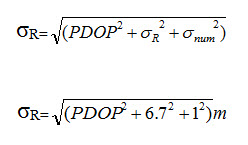
The term user equivalent range error (UERE) refers to the error of a component in the distance from receiver to a satellite. These UERE errors are given as ± errors thereby implying that they are unbiased or zero mean errors. These UERE errors are therefore used in computing standard deviations. The standard deviation of the error in receiver position, σ_rc, is computed by multiplying PDOP (Position Dilution of Precision) by σ_R, the standard deviation of the user equivalent range errors. σ_R is computed by taking the square root of the sum of the squares of the individual component standard deviations. PDOP is computed as a function of receiver and satellite positions.

User equivalent range errors (UERE) are shown in the Table 28.1. There is also a numerical error with an estimated value, σ_num, of about 1 meter. The standard deviations, σ_R, for the coarse/acquisition and precise codes are also shown in the table. These standard deviations are computed by taking the square root of the sum of the squares of the individual components (i.e., RSS for root sum squares). To get the standard deviation of receiver position estimate, these range errors must be multiplied by the appropriate dilution of precision terms and then RSS'ed with the numerical error. Electronics errors are one of several accuracy-degrading effects outlined in the table above. When taken together, autonomous civilian GPS horizontal position fixes are typically accurate to about 15 meters (50 ft). These effects also reduce the more precise P(Y) code's accuracy. However, the advancement of technology means that today, civilian GPS fixes under a clear view of the sky are on average accurate to about 5 meters (16 ft) horizontally.

σ_R for the C/A code is given by:

The standard deviation of the error in estimated receiver position  σ_rc, again for the C/A code is given by:

The error diagram in the Fig. 28.2 shows the inter relationship of indicated receiver position, true receiver position, and the intersection of the four sphere surfaces.

 

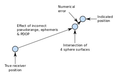
Fig. 28.2. Geometric Error Diagram Showing Typical Relation of Indicated Receiver Position, Intersection of Sphere Surfaces, and True Receiver Position in Terms of Pseudorange Errors, PDOP, and Numerical Errors. (Source: http://en.wikipedia.org/wiki/Error_analysis_for_the_Global_Positioning_System)

Fig. 28.3. Accuracy of navigation systems. (Source:http://en.wikipedia.org/wiki/Error_analysis_for_the_Global_Positioning_System)

Table 28.1 Sources of user equivalent range errors (UERE)

Sl. no.	Source	Effect(m)
1.	Signal arrival C/A	±3
2.	Signal arrival P(Y)	±0.3
3.	Ionospheric effects	±5
4.	Ephemeris errors	±2.5
5.	Satellite clock errors	±2
6.	Multipath distortion	±1
7.	Tropospheric effects	±0.5
8.	σR C/A	±6.7
9.	σR P(Y)	±6

(Source: http://en.wikipedia.org/wiki/Error_analysis_for_the_Global_Positioning_System)

28.2 Sources of GPS Error

The GPS signals sent from the SVs are subject to a variety of error sources before they are processed into a position and time solution in the receiver. As with most systems these error sources take the form of zero-bias noise, bias errors, and blunders. A number of conditions can reduce the accuracy of a GPS receiver. From a top-down perspective (from orbit down to ground level), the possible sources of trouble look like this:

1.    Selective Availability

Selective availability is the single largest source of C/A-code error. Y-code capable GPS receivers can remove SA with knowledge of the SA algorithm. SA takes the form of a slowly varying range error for each SV. SA introduces the largest bias errors in the Standard Positioning System accounting for most of the 100 meter (95 percent) error in the SPS. (Dana, 1997)

2.    Clock and Ephemeris Errors

Ephemeris errors occur when the satellite doesn’t correctly transmit its exact position in orbit. Clock and ephemeris data sets represent the difference between the SV clock and GPS time and permit the estimation of SV position at the time of transmission of the tracked codes. A GPS parameter, the User Range Accuracy (URA), is a range error estimate indicative of the “maximum value anticipated during each sub frame fit interval with uniform SA levels invoked” (Anon 1995, 35). The URA is transmitted as an integer power of two. Although the URA is not specified as a definite indicator of SA error magnitude, for a Block II SV affected by SA, a URA of 32 meters is common (Dana, 1997).

3.     Ionospheric Delays

The ionosphere starts at about 43–50 miles above the Earth and continues for hundreds of miles. Satellite signals traveling through the ionosphere are slowed down because of plasma (a low density gas). Although GPS receivers attempt account for this delay, unexpected plasma activity can cause calculation errors. (Dana, 1997)

A major source of bias error is the delay of the GPS carrier signals as they pass through the layer of charged ions and free electrons known as the ionosphere. (Dana, 1997). Varying in density and thickness as it rises and falls (50 to 500 kilometers) due to solar pressure and geomagnetic effects, the ionosphere can delay the GPS signals by as much as 300 nanoseconds (100 meters) (Klobuchar 1982). The diurnal (24-hour) changes in the ionosphere cause the largest variations in delay. At night the delay is at a minimum and the thinner and higher night-time ionosphere is more easily modeled than the less dense and thicker layer during the day. The signals from SVs at low elevation angles with respect to the local horizon experience the largest delays as the signal passes through more ionosphere than if the SV were directly overhead. Using the P-code, or special codeless (signal-squaring) techniques, the delay through the ionosphere can be computed by a receiver capable of measuring the phase delay difference between the code carried on the L1 and L2 signals (Dana, 1997). These dual frequency methods result in a substantial reduction of the ionospheric bias, making it possible to transfer sub-nanosecond clock offset measurements over thousands of kilometers (Dunn and others 1993, 174). For a single frequency (L1) C/A-code receiver the ionospheric delay can be estimated from the ionospheric delay model broadcast by the SVs. The Master Control station calculates the parameters for delay using a cosine model that computes delay for a given local time-of-day and the elevation angle for the path from the receiver to an SV. Some users compute an ionospheric delay estimate from their own models. Using the broadcast model under normal conditions removes about half of the error (Fees and Stephens 1987) leaving a residual error of around 60-90 nanoseconds during the day and 10 to 20 nanoseconds at night (Knight and Rhoades 1987). Signals from SVs at high elevation angles experience smaller delays, but use of the broadcast model under abnormal conditions can occasionally introduce more error than that caused by the actual delay. (Dana, 1997)

4.     Tropospheric Delays

The troposphere is the lowest region in the Earth’s atmosphere and goes from ground level up to about 11 miles. Variations in temperature, pressure, and humidity all can cause variations in how fast radio waves travel, resulting in relatively small accuracy errors. GPS signal delays through the troposphere, the layer of atmosphere usually associated with changes in weather (from ground level up to 8 to 13 kilometers), are subject to local conditions and are difficult to model. GPS does not broadcast a tropospheric correction model but several such models have been developed. Some receivers make a limited model available that computes tropospheric delay from receiver height and SV elevation angle using nominal atmospheric parameters. (Dana, 1997). Because accurate tropospheric delay models (Turner and others 1986) require local pressure, temperature and humidity (PTH) data as well as receiver height and elevation angle to the SV, these models are difficult to apply in real-time situations. The errors introduced by an unmodeled troposphere may be as much as 100 nanoseconds at low elevation angles (less than 5 degrees), but are more typically in the 30 nanosecond range (Knight and Rhoades 1987). Residuals after application of a simple, no-PTH, model (Gupta 1980) are in the 10 nanosecond range.

5.     Multipath

When a satellite signal bounces off a hard surface (such as a building or canyon wall) before it reaches the receiver, a delay in the travel time occurs, which causes an inaccurate distance calculation. Multipath interference, caused by local reflections of the GPS signal that mix with the desired signal, slowly introduces varying bias errors of one to two nanoseconds for navigation receivers aboard aircraft in flight. For land-based systems, local conditions and exact antenna placement can result in errors of up to 150 nanoseconds. (Dana, 1997). Nominal errors for land-based receivers are in the 30 nanosecond range (Braasch, 1995). Careful attention to antenna placement, antenna design, the use of choke rings, and the use of materials that absorb GPS radio-frequency signals can mitigate much of the potential multipath interference, but these measures must be carefully designed to allow for the different multipath reflections from the constantly changing SV elevations and azimuths. In many applications it is difficult or impossible to completely eliminate multipath errors. (Dana, 1997)

6.   GPS Signal Noise

Propagation of the GPS signals from the SV to the receiver introduces noise from galactic sources, ionospheric scintillations, and cross correlation from other GPS SV signals that results in small noise (zero bias) errors in the three nanosecond range. (Dana, 1997)

7.    Receiver Noise and Delays

Receiver noise can introduce two to three nanoseconds of zero bias noise in the timing measurements of a GPS receiver. Delays within a receiver can be calibrated by the manufacturer, but if receiver delays change with temperature or change differently between channels of a multi-channel receiver, timing bias errors can result. Antenna cable delays must be recomputed or calibrated if cable lengths change or cables of different materials are used. (Dana, 1997). There have been reports of cable delays being both temperature and signal strength dependent (Lewandowski, Petit and Thomas 1991, 5). Manufacturers can provide cable delays for the equipment they supply. (Dana, 1997)

8.  Receiver Oscillator Errors

While precise time standards at the Control and Space Segments of GPS are designed to keep user clock requirements to a minimum, receiver oscillators must provide enough stability to insure that they can be rated properly by GPS receiver software and that they provide a low noise timing reference. This is sometimes difficult to accomplish in high dynamic environments or when the receiver internal temperatures cannot be controlled or compensated for. (Dana, 1997)

9.   SV clock errors 

The uncorrected by Control Segment can result in one meter errors in position. (Dana, 1997)

10.  Geometric Dilution of Precision

Geometric Dilution of Precision (GDOP) is a measurement of the sensitivity of a receiver position or time estimate to changes in the geometric relationship between the receiver position and the positions of all of the SVs used to form the position or time estimate. If the SVs used for a navigation solution were all in about the same place in the sky, directly above a receiver position, for instance, the position solution for height would be less sensitive to pseudo-range changes than would the poorly defined (diluted) solution for horizontal position. If the SVs were distributed around the field of view of the receiver, horizontal and vertical positioning would be more equally sensitive to pseudo-range changes. GDOP is a dimensionless multiplier that can be used to estimate the effect of pseudo-range errors on a complete position and time solution. The single GDOP parameter is the square root of the sum of the diagonal terms of the covariance matrix that is formed from the inverse of the matrix of directional derivatives for each of the SV positions and pseudo-ranges used in the position solution. For a specified receiver position and a set of SVs, GDOP can be separated into three-dimensional position (PDOP) or spherical (SDOP) dilution, two-dimensional horizontal (HDOP), or one dimensional vertical (VDOP) or time (TDOP) estimates. These separate components of GDOP are formed from covariance terms and so are not independent of each other. A high TDOP (time dilution of precision) in a navigation receiver will eventually influence position errors as erroneous receiver clock bias estimates are used to correct pseudo-range measurements.

The computation of geometric dilution of precision involves many numerical equations. Computations were provided to show how PDOP was used and how it affected the receiver position error standard deviation. When visible GPS satellites are close together in the sky (i.e., small angular separation), the DOP values are high; when far apart, the DOP values are low. Conceptually, satellites that are close together cannot provide as much information as satellites that are widely separated. Low DOP values represent a better GPS positional accuracy due to the wider angular separation between the satellites used to calculate GPS receiver position. HDOP, VDOP, PDOP and TDOP are respectively Horizontal, Vertical, Position (3-D) and Time Dilution of Precision. (Dana, 1997)

11.  Poor satellite coverage

When a significant part of the sky is blocked, your GPS unit has difficulty receiving satellite data. Unfortunately, you can’t say that if 50 percent (or some other percentage) of the sky is blocked, you’ll have poor satellite reception; this is because the GPS satellites are constantly moving in orbit. A satellite that provides a good signal one day may provide a poor signal at the exact same location on another day because its position has changed and is now being blocked by a tree. The more open sky you have, the better the chances of not having satellite signals blocked.

Building interiors, streets surrounded by tall buildings, dense tree canopies, canyons, and mountainous areas are typical problem areas. (McNamara, 2004)

28.3 Accuracy of GPS

The errors can be compensated for (in great part) using differential GPS measurement methods. In this approach, simultaneous measurements are made by a stationary base station receiver (located over a point of precisely known position) and one (or more) roving receivers moving from point to point. The positional errors measured at the base station are used to refine the position measured by the rover(s) at the same instant in time. This can be done either by bringing the data from the base and rover together in a post-processing mode after the field observations are completed or by instantaneously broadcasting the base station corrections to the rovers. The latter approach is termed real-time differential GPS positioning. (Lillesand and Keiffer, 2004)

In general, each GPS satellite continuously transmits a microwave radio signal composed of two carriers, two codes, and a navigation message. When a GPS receiver is switched on, it will pick up the GPS signal through the receiver antenna.

Once the receiver acquires the GPS signal, it will process it using its built-in software. The partial outcome of the signal processing consists of the distances to the GPS satellites through the digital codes (known as the pseudoranges) and the satellite coordinates through the navigation message.

Theoretically, only three distances to three simultaneously tracked satellites are needed. In this case, the receiver would be located at the intersection of three spheres; each has a radius of one receiver-satellite distance and is centered on that particular satellite. From the practical point of view, however, a fourth satellite is needed to account for the receiver clock offset. The accuracy obtained with this method was limited to 100m for the horizontal component, 156m for the vertical component, and 340 ns for the time component, all at the 95% probability level. This low accuracy level was due to the effect of the so-called selective availability, a technique used to intentionally degrade the autonomous real-time positioning accuracy to unauthorized users. To further improve the GPS positioning accuracy, the so-called differential method, which employs two receivers simultaneously tracking the same GPS satellites, is used. In this case, positioning accuracy level of the order of a sub-centimeter to a few meters can be obtained.

According to the government and GPS receiver manufacturers, the GPS unit is accurate within 49 feet (that’s 15 meters for metric-savvy folks). If the GPS reports that we’re at a certain location, we can be reasonably sure that we’re within 49 feet of that exact set of coordinates. GPS receivers tell us how accurate our position is. Based on the quality of the satellite signals that the unit receives, the screen displays the estimated accuracy in feet or meters.

Accuracy depends on:

a)     Receiver location

b)    Obstructions that block satellite signals

Even if we’re not a U.S. government or military GPS user, we can get more accuracy by using a GPS receiver that supports corrected location data. Corrected information is broadcast over radio signals that come from either

a)     Non-GPS satellites

b)    Ground-based beacons

Two common sources of more accurate location data are

a)     Differential GPS (DGPS)

b)    Wide Area Augmentation System (WAAS)

Source: McNamara, J., 2004, GPS for Dummies, Wiley Publishing, Inc., Indianapolis, Indiana, pp. 49-68. (McNamara, 2004)

28.3.1 Differential Techniques

For both code-phase tracking navigation and carrier-phase tracking survey techniques, bias errors can be removed or mitigated by the use of differential techniques. (Dana, 1997)

• Post-Processed Precise Ephemerides

Some GPS position techniques make use of precise ephemeris data that is published by public and private agencies from the measurement of GPS signals at multiple reference locations. These data sets are available from agencies such as the International GPS Service for Geodynamics and the U. S. National Geodetic Survey within a few days or weeks of their reference times. (Dana, 1997). Precise orbital data used in post-processed position solutions can improve the accuracy of both code and carrier-phase derived solutions (Lewandowski, Petit, and Thomas 1991, 3). (Lewandowski, Thomas, 1991)

• Differential GPS (DGPS)

Selective Availability errors are correlated to a large extent for receivers within a few hundred kilometers of each other. For code tracking techniques, the ionospheric errors can be considered common to sites separated by a few hundred kilometers. Carrier tracking receivers can resolve differences in integer carrier wavelengths for receivers located within twenty to thirty kilometers of each other. Differential GPS (DGPS) is based on the assumption that bias errors common to two receivers, one a reference receiver at a known location, the other a remote receiver at an unknown location, can be measured at the reference receiver and applied to the remote receiver. DGPS techniques are based on the correction of individual SV pseudo-ranges or SV carrier phase measurements. While it would be possible to apply a simple position correction from the reference receiver to the remote, both receivers would have to be tracking the identical set of SVs with identical GDOP components for the position solution transfer to be effective. While this common-view technique can work for specialized applications were great care is taken to track the same set of SVs over identical time periods, for general-purpose DGPS positioning this technique is not recommended. In most DGPS positioning systems the bias errors in each SV signal are measured at the reference receiver, which either sends corrections in real time to the remote receiver, or records the corrections for later application in post-processing software. In the remote receiver, or in post-processing software, the pseudo-range corrections are applied to the remote measurements prior to the formation of a position solution. (Dana, 1997)

• Interferometric Processing

Measurements of crustal movements of the earth, earthquake fault line monitoring, and precise position transfer to isolated islands are possible using GPS interferometric techniques. In these special-purpose differential techniques, recordings of the pseudorandom codes and carrier-phase measurements on the GPS signals from distant sites are correlated and used along with precise ephemeris data in a post-processed mode to achieve position estimates in the centimeter range over thousands of kilometers. Global networks of carrier-phase tracking receivers are used in these processes. (Dana, 1997)

• Common View

Not usually suitable for control of real-time systems or for positioning systems, common view measurements are often used to transfer precise time from one location to another. Two receivers, both at known fixed positions, measure signals from a single satellite over the same carefully chosen observation period. Both receivers collect and filter data with the same methods. (Dana, 1997) The clock errors at the location with the reference standard are then transmitted to the other site, allowing the remote site to correct a clock with accuracies that have been obtained in the 8 nanosecond range for 1000 kilometer baselines and 10 nanoseconds for 5000 kilometer baselines (Lewandowski 1993, 138) (Lewandowski 1993, 138).

Selective Availability

GPS has the proven potential to disseminate time and time intervals with accuracies of around 100 nanoseconds. Frequency control can be established globally to accuracies of a few parts in 10-12. The Block I satellites, placed in orbit during the 1970s and 1980s, gave promising results for worldwide time and frequency users. The new Block II satellites being launched now, however, have provisions for the implementation of selective availability (SA). SA is the intentional degradation of GPS signals and navigation messages to limit the full accuracy of the system to authorized users. Implemented last March, SA seriously affects both the time and frequency accuracies of GPS. Early tests indicate that accuracies are degraded from errors of approximately 100 nanoseconds to errors of approximately 500 nanoseconds. Fig. 28.4 shows actual results of selective availability on timing accuracies during a three-day period. Frequency control accuracies are reduced to a few parts in 10^-10. (Dana and Bruce, 1990)

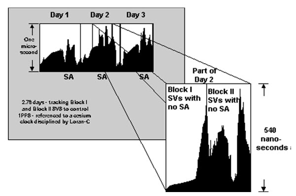
Fig. 28.4. Selective availability effect on 1PPS control.

(Source: Dana and Bruce, 1990)

Because most authorized users of GPS are in the military or otherwise affiliated with the Department of Defense (DoD), many non DoD time and frequency users are already being denied access to the accurate signals on the Block II satellites. Because the Block I satellites are nearing the end of their useful life and the current DoD policy is to continue SA, many users are turning back to cesium clocks and systems like Loran-C. To date, DoD has denied requests for undegraded signals from certain SVs, which would allow for accurate time and frequency use without compromising the agency's goal of degrading position accuracy. Fortunately, use of common-view, cornmon-mode techniques can considerably reduce SA's effects on time transfer. The technique assumes that SA produces similar errors in both receivers involved in the time transfer. With careful time synchronization of the viewing window at the reference and common-view receivers, and with identical code phase-averaging techniques, the corrections transmitted from the reference station will remove most of the SA errors at the remote receiver site. (Dana and Bruce, 1990)

Table 28.2. shows the accuracy we can expect from a GPS receiver. These numbers are guidelines; at times, we may get slightly more or less accuracy.

	GPS Accuracy
GPS Mode	Distance in Feet	Distance in Meters
GPS without SA	49	15
GPS with DGPS	10–16	3–5
GPS with WAAS	10	3

(Source: McNamara, 2004)

Signal arrival time measurement

The position calculated by a GPS receiver requires the current time, the position of the satellite and the measured delay of the received signal. The position accuracy is primarily dependent on the satellite position and signal delay.

To measure the delay, the receiver compares the bit sequence received from the satellite with an internally generated version. By comparing the rising and trailing edges of the bit transitions, modern electronics can measure signal offset to within about one percent of a bit pulse width, , or approximately 10 nanoseconds for the C/A code. Since GPS signals propagate at the speed of light, this represents an error of about 3 meters.

This component of position accuracy can be improved by a factor of 10 using the higher-chiprate P(Y) signal. Assuming the same one percent of bit pulse width accuracy, the high-frequency P(Y) signal results in an accuracy of  or about 30 centimeters.

The U.S. Coast Guard operates the most common differential GPS correction service. This system consists of a network of towers that receive GPS signals and transmit a correction signal using omni-directional beacon transmitters. In order to receive the correction information, users must have a differential beacon receiver and beacon antenna in addition to their GPS. No such additional equipment is necessary with receivers that include Wide Area Augmentation System (WAAS) capability. (http://en.wikipedia.org/wiki/Error_analysis_for_the_Global_Positioning_System)

• WAAS

The WAAS consists of approximately 25 ground reference stations distributed across the United States that continuously monitor GPS satellite data. Two master stations, located on the East and West Coasts, collect the data from the reference stations and create a compo sited correction message that is location specific. This message is then broadcast through one of two geostationary satellites, satellites occupying a fixed position over the equator. Any WAAS-enabled GPS unit can receive these correction signals. The GPS receiver determines which correction data are appropriate at the current location.

The WAAS signal reception is ideal for open land, aircraft, and marine applications, but the position of the relay satellites over the equator makes it difficult to receive the signals when features such as trees and mountains obstruct the view of the horizon. In such situations, GPS positions can sometimes actually contain more error with WAAS correction than without. However, in unobstructed operating conditions where a strong WAAS signal is available, positions are normally accurate to within 3 m or better.

Paralleling the deployment of the WAAS system in North America are the Japanese Multi-functional Satellite Augmentation System (MSAS) in Asia and the European Geostationary Navigation Overlay Service (EGNOS) in Europe. Eventually, GPS users will have access to these and other compatible systems on a global basis.

Till the year 2002, the U.S. Global Positioning System has only one operational counterpart, the Russian GLONASS system. However, a fully comprehensive European global satellite navigation system, Galileo, is scheduled for operation in the coming years. The future for these and similar systems is an extremely bright and rapidly changing one. (Lillesand and Keiffer, 2004)

28.4 Application of Global Positioning System

There are so many devices made with the implementation of Global Positioning System. Google Earth is the most famous application that uses the signals received by the GPS receivers. It enables public also to access the maps which tell the users about the locations all around the world.3DEM is freely available software that will create 3D terrain scenes and flyby animations and export GIS terrain data files using any of the following freely available terrain data as a source. People use Global Positioning System for several uses. A research published states that the percentage of uses for each several requirement is as follows.

• Car navigation 37%

• Hand held 26%

• Tracking 10%

• GIS 8%

• Survey 7%

• Manufacturing 7%

• Vessel Voyage 2%

• Military Related 1%

United States and European countries show a rapid growth in using GPS for the car navigations and the number of GPS equipped mobile phone usage. Those facts prove that the Global Positioning System helps many people in many other ways.

Most people who have used a GPS probably can’t imagine any limit to its applications. Even if its shortcomings are grievous (it can’t be used indoors, nor very well in a forest, or where there are many tall buildings or cliffs), solutions have been developed to these problems. Usually these solutions involve broadcasting radio signals or pseudo-GPS signals that are highly accurate. The configuration of these systems is very complicated and requires large institutional investments. Most are made by governments. For instance, the European Union is developing a high-accuracy network (along the lines of the U.S. WAAS) for navigation purposes. Even if a GPS receiver lacks the ability to use these extra networks, GPS can still be used in a number of applications, some of which are described here.

28.4.1 GPS-supported ground surveys

Ground surveys are generally carried out for cadastral purposes of larger areas in terrain, where visibility requirements of the boundaries prohibit the use of photogrammetric techniques. They may also be preferable in countries where photo-adjudication is not accepted due to accuracy concerns. In Europe, cadastral data are already existent. Therefore, a survey cost comparison with photogrammetric methods is not useful there. However, in a number of development projects, ground survey costs per parcel, including the land registration or land titling aspects, have been established.

In Albania, a new cadaster has been established by European funding at a cost of $5 per parcel. The procedure used was aerial photography–aerial triangulation–digital elevation model–digital orthophotos generation followed by public photo adjudication process. In Georgia, a large German technical cooperation project was carried out by GPS-supported electronic tacheometers at a cost of $10 per parcel.

A survey crew is able to measure about fifty parcels per day. In doing so, it has been proved useful to support the ground surveys with aerial photos or orthophotos. For this purpose, ‘digital plane tables’ in the form of large-screen PDAs may be used which record the measured GPS or electronic tacheometer measurements on the screen. These data are superimposed with preprepared (ortho) photographic data on the screen, which helps to identify points to be measured terrestrially. A ‘digital plane table’ costs about $10 000.

An urban area of 250 km² has about 80 000 parcels. The cost of surveying these terrestrially would therefore be $800 000, which is about the same as the photogrammetric line mapping cost at the scale 1:1000, but about four times as much as the photogrammetric mapping cost at the scale 1:2000. This corresponds to a terrestrial survey cost of $3200/km².

28.4.2 Mapping and geographic information systems (GIS)

Most mapping grade GPS receivers use the carrier wave data from only the L1 frequency, but have a precise crystal oscillator which reduces errors related to receiver clock jitter. This allows positioning errors on the order of one meter or less in real-time, with a differential GNSS (Global Navigation Satellite System) signal received using a separate radio receiver. By storing the carrier phase measurements and differentially post-processing the data, positioning errors on the order of 10 centimeters are possible with these receivers.

28.4.3 Geophysics and geology

High precision measurements of crustal strain can be made with differential GNSS by finding the relative displacement between GNSS sensors. Multiple stations situated around an actively deforming area (such as a volcano or fault zone) can be used to find strain and ground movement. These measurements can then be used to interpret the cause of the deformation, such as a dike or sill beneath the surface of an active volcano.

28.4.4 Archeology

As archaeologists excavate a site, they generally make a three-dimensional map of the site, detailing where each artifact is found.GPS capable of precise tracking of carrier phases for all or most of available signals in order to bring the accuracy of relative positioning down to cm-level values required by these applications.

28.4.5 GPS Tracking

In fact, it is this use which represents the simplest form of GPS tracking. The user is able, using a portable GPS device, to keep a track of where they have been, in order to be able to either retrace their steps, or follow the same path again in the future. When combined with other technologies such as GPS phones, this also gives the possibility for other users of GPS to follow in the footsteps of the initial user; which can be a useful application of GPS tracking for field activities.

Where GPS tracking comes into its own, however, is when it is combined with other broadcast technologies such as radio. GPS watches, for example, can be fitted with a GPS receiver which is capable of calculating its position, whilst also broadcasting that using a miniature radio transmitter. The signal is relayed to a central command center equipped with GPS software systems which can track the position of the wearer, and either store it as a path, or relay that information to a third party. That third party could be an anxious parent, or the police. In fact there are a variety of GPS phones and wristbands which are sold in conjunction with a service which enables third parties to find out where their charges are at any time of the day or night.

28.4.6 GPS Vehicle Tracking

This is particularly useful when using GPS units attached to vehicles which have distinctive identification such as chassis numbers. The same principle applies as for a GPS tracking device designed to be worn by a human, except that the GPS is integrated within the vehicular electronics. This serves two purposes. On the one hand, it provides the driver with an integrated GPS system, without the necessity to purchase a car navigation system, or a PDA-based GPS system, whilst also offering the possibility to relay that information via a radio or mobile phone transmitter. In fact, these systems have already been tried in the field, primarily as a vehicle locator in the event that the vehicle to which the GPS vehicle tracking system is attached is stolen. The police, once informed, can find out from the control center where the vehicle is, and proceed to track it physically. A useful consequence of being able to use GPS vehicle tracking to locate a vehicle is that the manufacturer can also use the information to alert the driver as to when they near a service center. If, along with the GPS coordinates, the system relays telemetry information such as the status of the engine, time since the last service, or even information not relating to defects, the receiver of this information can make a decision as to what kind of alert to pass on to the driver. More and more people have used GPS-based systems in cars; many more have benefited from the use of GPS in cars, buses, trains, and trucks. The GPS receiver may be hidden in the dashboard, but may be critical for the taxi company to find out which taxi is closest to you when you call for a pickup. A GPS receiver can help a trucking company better organize deliveries to minimize the fuel used. A bus may have a GPS installed to help the bus company indicate to passengers how long they need to wait for the next one. Navigation systems are used for more than vehicles on land. They are also widely used for nautical and aeronautical navigation. They have become for many sailors irreplaceable because they work regardless of the weather and can easily be combined with computerized chart information. Almost all planes use, or will use, GPS. Together with high-precision positional trans-mission, planes can use GPS-based systems to land in any weather with centimeter precision.

28.4.7 Coordinated Tracking

This also opens up the possibility to allow for coordinated vehicle tracking, in which GPS tracking is used to share location information between several vehicles, all pursuing the same end goal. It is an approach that has been used successfully in conjunction with GPS fish-finder units which help fisherman to locate, track and catch schools of fish. These units are more sophisticated than the average GPS unit, having other features such as depth gauges, tide time information and so forth. The basic GPS functionality is the same however, and units can either share that information with each other, or a central point. The central point can also be one of the fishing vessels, and it has on-board computer systems capable of reconciling all the locator information along with a map, thus allowing the different vessels to coordinate their actions. This also has military applications, of course, where units can share, in real time, information about their location, even when line-of-sight is no longer possible. In the past, this was done by relaying often inaccurate map co-ordinate estimations; now the locations can be called in with high absolute accuracy.

28.4.8 Consumer GPS Tracking

Despite its’ hi-tech military and commercial fishing applications, as well as use in aviation GPS, the principal application of GPS tracking will be in providing an enabling technology to augment existing systems. These systems will include cell phones and vehicles, usually in conjunction with a central point of service designed to keep track of the location.

28.4.9 Use of GPS to determine well location

There is typically a lot of good geologic and hydrologic information contained on the well log and drilling report forms. In order for this data to be used for mapping purpose and some regulatory programs, the exact location of well has to be known. GPS have made it possible.

28.4.10 Weather Prediction Improvements

Measurement of atmospheric bending of GNSS satellite signals by specialized GNSS receivers in orbital satellites can be used to determine atmospheric condition such as air density, temperature, moisture and electron density. Such information from a set of six micro-satellites, launched in April 2006, called the Constellation of Observing System for Meteorology, Ionosphere and Climate COSMIC has been proven to improve the accuracy of weather prediction models.

28.4.11 Photographic Geocoding

Combining GNSS position data with photographs taken with a (typically digital) camera, allows one to view the photographs on a map or to lookup the locations where they were taken in a gazetteer. It's possible to automatically annotate the photographs with the location they depict by integrating a GNSS device into the camera so that co-ordinates are embedded into photographs as Exif (Exchangeable image file format) metadata. Alternatively, the timestamps of pictures can be correlated with a GNSS track log.

28.4.12 Marketing

Some market research companies have combined GIS systems and survey based research to help companies to decide where to open new branches, and to target their advertising according to the usage patterns of roads and the socio-demographic attributes of residential zones.

28.4.13 Social Networking

Cellular phones equipped with GPS technology, offering the ability to pinpoint friends on custom created maps, along with alerts that inform the user when the party is within a programmed range.

28.4.14 Altitude Information

GPS has transformed how altitude at any spot is measured. GPS uses an ellipsoid coordinate system for both its horizontal and vertical datums. An ellipsoid—or flattened sphere—is used to represent the geometric model of the earth.

28.4.15 Application to Water Resources

In an effort to protect water resources, GPS is being used to collect the coordinates for well heads as part of the Well Head Protection Program. GPS has also been used to produce coordinates for potable surface water intakes, and reservoir boundaries. To more effectively manage regulatory permits across the various environmental permitting programs, GPS is being used to collect coordinates for facilities that have permits. These include facilities that discharge to surface water, ground water, air, store hazardous waste onsite and/or have underground storage tanks. Environmental monitoring programs are using GPS to generate coordinates for monitoring stations. Water monitoring programs have been determining coordinates of sampling stations for existing water quality monitoring networks. Should a major oil spill occur in their waters, coordinates for the spill location and aerial extent of the plume could be collected. In short order, an effective booming strategy could be developed to protect environmentally sensitive areas in the region of the spill. In the event of a major natural disaster, GPS can be used to assist in the damage assessment and inventory.

GPS Techniques for Water Stage Measurement and River Slope Calculation Wetland Area

Study of river basin many times involves difficulties of making use of hydrological data such as river stage height due to inaccessibility and political boundaries. The slope of river is very important hydrological data especially from point of view of hydrologic and hydrodynamic models calibration. These specific hydrologic applications need calculation of local changes of water level and slope. Traditionally slope is calculated using data available from water gauge which are always insufficient and the distance between two successive gauge stations varies from few to several kilometers. For hydrodynamic model calibration the water stage determined based on water level measured should be within few hundred meters. In natural river valley such detailed measurements are difficult to perform by use of classical geodetic leveling technique; in case of marginal river wetland it is even impossible, because of harsh measuring condition such as:

• Disturbance of natural vegetation.

• Many oxbow and wetland areas.

• Unstable organic ground.

• Very few network coordination points.

The GPS technique seems to be optimal tool for altitude measurement in wetlands. The average vertical measurement error for DGPS is about 3m which is sufficient for river slope calculation. GPS become not only accurate but also very fast measurement technique. Moreover GPS technique allows performing high accuracy measurement of all three co-ordinates including altitude, easy and fast way. The DGPS definitely can be used for hydrologic application in various water-bodies.

Use of GPS receivers as a soil moisture network for water cycle studies

Soil moisture is fundamental to land surface hydrology, affecting flooding, groundwater recharge, and evapotranspiration [Viterbo and Betts, 1999]. It also influences weather and climate via its influence on turbulent andradiative fluxes between the land surface and atmosphere [Entekhabi and Rodriguez-Iturbe, 1994]. The global distribution and temporal variations of soil moisture are sought both  for analyses and modeling purposes. Soil moisture is measured in situ at many locations, both as part of individual studies or as part of monitoring networks.

Measurements of soil moisture, both its global distribution and temporal variations, are required to study the water and carbon cycles. Signals routinely recorded by Global Positioning System (GPS) receivers for precise positioning applications can also be related to surface soil moisture variations. Various studies depicted significant correlation between the result obtain from GPS network and soil moisture fluctuation measured in the top 5 cm of soil with conventional sensors.

28.4.16 Application to Agriculture

Global positioning systems (GPS) are widely available in the agricultural community. Farm uses include:

• Mapping yields (GPS + combine yield monitor)

• Variable rate planting (GPS + variable rate planting system)

• Variable rate lime and fertilizer application (GPS + variable rate controller)

• Field mapping for records and insurance purposes (GPS + mapping software)

• Parallel swathing (GPS + navigation tool).

The Global Positioning System (GPS) provides opportunities for agricultural producers to manage their land and crop production more precisely. Common names for general GPS applications in farming and ranching include precision agriculture, site-specific farming and prescription farming. GPS applications in farming include guidance of equipment such as sprayers, fertilizer applicators and tillage implements to reduce excess overlap and skips. They can also be used to precisely locate soil-sampling sites, map weed, disease and insect infestations in fields and apply variable rate crop inputs, and, in conjunction with yield monitors, record crop yields in fields.

GPS and associated navigation system are used in many types of agricultural operations. These          systems are useful particularly in applying pesticides, lime, and fertilizers and in tracking wide planters/drills or large grain-harvesting platforms. GPS navigation tools can replace foam for sprayers and planter/drill-disk markers for making parallel swaths across a field. Navigation systems help operators reduce skips and overlaps, especially when using methods that rely on visual estimation of swath distance and/or counting rows. This technology reduces the chance of misapplication of agrochemicals and has the potential to safeguard water quality. Also, GPS navigation can be used to keep implements in the same traffic pattern year-to-year (controlled traffic), thus minimizing adverse effects of implement traffic.

Yield Monitoring Systems

Yield monitoring systems typically utilize a mass flow sensor for continuous measuring of the harvested weight of the crop. The sensor is normally located at the top of the clean grain elevator. As the grain is conveyed into the grain tank, it strikes the sensor and the amount of force applied to the sensor represents the recorded yield. While this is happening, the grain is being tested for moisture to adjust the yield value accordingly. At the same time, a sensor is detecting header position to determine whether or not yield data should be recorded. Header width is normally entered manually into the monitor and a GPS, radar or a wheel rotation sensor is used to determine travel speed. The data is displayed on a monitor located in the combine cab and stored on a computer card for transfer to an office computer for analysis. Yield monitors require regular calibration to account for varying conditions, crops and test weights. Yield monitoring systems cost approximately $3,000 to $4,000, not including the cost of the GPS unit.

Field Mapping with GPS and GIS

GPS technology is used to locate and map regions of fields such as high weed, disease and pest infestations. Rocks, potholes, power lines, tree rows, broken drain tile, poorly drained regions and other landmarks can also be recorded for future reference. GPS is used to locate and map soil-sampling locations, allowing growers to develop contour maps showing fertility variations throughout fields. The various datasets are added as map layers in geographic information system (GIS) computer programs. GIS programs are used to analyze and correlate information between GIS layers.

Precision Crop Input Applications

GPS technology is used to vary crop inputs throughout a field based on GIS maps or real-time sensing of crop conditions. Variable rate technology requires a GPS receiver, a computer controller, and a regulated drive mechanism mounted on the applicator. Crop input equipment such as planters or chemical applicators can be equipped to vary one or several products simultaneously. Variable rate technology is used to vary fertilizer, seed, herbicide, fungicide and insecticide rates and for adjusting irrigation applications.

Precision Farming

Location coordinate information is needed in precision agriculture to map in-field variability, and to serve as a control input for variable rate application. Differential global positioning system (DGPS) measurement techniques compare with other independent data sources for sample point location and combine yield mapping operations. Sample point location can be determined to within 1m (3ft) 2dRMS using CIA code processing techniques and data from a high-performance GPS receiver. Higher accuracies can be obtained with carrier phase kinematic positioning methods, but this required more time. Data from a DGPS CIA code receiver are accurate enough to provide combine position information in yield mapping. However, distance data from another source, such as a ground-speed radar or shaft speed sensor, needed to provide sufficient accuracy in the travel distance measurements used to calculate yield on an area basis.

Precision farming, sometimes called site-specific agriculture, is a strategic task for agriculture: indeed it has the potential to reduce costs through more efficient and effective applications of crop inputs; it can also reduce environmental impacts by allowing farmers to apply inputs only where they are needed at the appropriate rate. Precision farming requires the use of new technologies, such as GPS, environmental sensors, satellites or aerial images and GIS to asses and understands variations. The various research deals with potentialities and limits of GPS for navigation in agricultural applications. GPS needs for farming applications are:

• Low cost in order to allow farmers to buy GPS technologies;

• High precision in order to reduce the use of pesticides and fertilizers by means of an exact track.

At first, static and kinematic tests needed to be performed, simulating the typical behavior of an agricultural vehicle and using different kinds of GPS receivers and navigation software. The experimental results are presented: particularly, advantages and disadvantages of the popular Kalman filtering on trajectories are discussed. Starting from the analyses of the previous results, and taking into account the typical user requirements, a preliminary design for a new prototype has been done; particularly, both needed instrumentations and their costs and a proposal of a new navigation algorithm will be presented.

Precision farming is a method of crop management by which areas of land within a field may be managed with different levels of input depending upon the yield potential of the crop in that particular area of land. The benefits of so doing are two fold:

• The cost of producing the crop in that area can be reduced.

• The risk of environmental pollution from agrochemicals applied at levels greater than those required by the crop can be reduced.

Precision farming is an integrated agricultural management system incorporating several technologies. The technological tools often include the global positioning system GPS, geographical information system GIS, remote sensing, yield monitor and variable rate technology. The paper talks about the use of GPS to support agricultural vehicle guidance. Equipment for this purpose consists on a yield monitor installed: the system supports human guide by means of a display mapping with a GIS the exact direction produced by GPS receiver put on vehicle top: the driver follows it to cover in an optimal path the full field. GPS receivers for this applications require, not only an high accuracy to ensure the reduction of input products, but even an easy and immediate way of use for farmers; without forgetting low costs.

Obviously the technology to achieve high precision still exists but it is too expensive and difficult to use for not skilled people. Survey modality usually adopted in agricultural applications is real time kinematic positioning, DGPS RTK, which enable to have a good accuracy by means of corrections received. In this experimentation the aim is to obtain a sub-metric accuracy using low cost receivers, which can provide only point positioning. These receivers have been developed for maritime navigation purposes; our aim is their optimization in order to apply them for land navigation in particular for farming activities. Some tests using these receivers were carried out, but results were not satisfying and probably the reason has to be assigned to the implementation of a Kalman filtering inside the receiver software. This is the starting point for a new project, at the moment still in progress, which aim to develop a new algorithm based on Kalman filter. Its purpose is to improve low cost receiver outputs in order to optimize trajectories and to reach needed accuracy in vehicle positioning during agricultural activities.

28.4.17 Others

• Hiking: More and more hikers turn to GPS to help them find out more exactly where they are and to help them to plan a route before they go. GPS may not be reliable in canyons or along steep cliffs, but in most situations and weather it provides accurate positional information. Some map makers have started to change their map designs to make it easier for hikers to use. Some tourist areas offer GPS for people to help them follow a certain tour.

• Aids for the Visually Impaired: Combined with acoustic or tactile signaling devices, GPS can be used to help visually impaired people find their way in new settings and navigate places that rapidly change—for example, a state fair or a college campus, as was done by Professor RegGolledge and others at the University of California at Santa Barbara

Keywords: Global Positioning System, Pseudoranges, DOP, PDOP, GDOP, SDOP, HDOP, VDOP, TDOP, DGPS, WAAS, UERE, URA, SV, SA, PTH, MSAS, EGNOS, GLONASS.

References

• Anon. 1995, Global Positioning System Standard Positioning Service Signal Specification. 2nd. edition. United States Coast Guard Navigation Center.

• Biagi, L. et. al, “GPS Navigation for Precision farming.”Ohio Department of Natural Resources,“Use of Global Positioning System (GPS) to determine well location for Ohio’s water  well log and drilling report.”

• Braasch, Michael S., 1995, Isolation of GPS multipath and receiver tracking errors. In Navigation: Journal of the Institute of Navigation. 41, no. 4: 415-434.

• Cheng, K. (2005).“Analysis of water level measurement using GPS.” Report No. 476, Ohio State University.

• Dana  Peter H. and Bruce M. Penrod, 1990, “The role of GPS in precise time and frequency dissemination,” Timing and frequency, GPS World.

• Dana, Peter H. 1997, Global Positioning System Overview, NCGIA Core Curriculum in GIScience, http://www.ncgia.ucsb.edu/giscc/units/u017/u017.html, posted August 28, 1997.

• Dana, Peter H., 1997, “Global Positioning System (GPS) Time   Dissemination for Real-Time Applications.” Real-Time systems, 12, pp. 9-40.

• Dunn and others. 1993, Time and position accuracy using codeless GPS. In 25th annual Precise Time and Time Interval (PTTI) applications and planning meeting. Marina Del Rey, CA, pp. 169-179.

• Fees, W. A. and S. G. Stephens, 1987, Evaluation of GPS ionospheric time-delay model. IEEE Transactions on Aerospace and Electronic Systems, AES-23, no. 3 (May).

• Gupta. S. K., 1980, Test and evaluation procedures for the GPS user equipment. Global Positioning System, Volume I, Washington, DC: Institute of Navigation.

• Harvey, F. (2008). “Surveying, GPS, Digitization” A Primer of GIS:Fundamental Geographic and Cartography Concepts. The Guilford press, New York.

• http://en.wikipedia.org/wiki/Global_Positioning_System

• http://notesofgenius.com/gps-applications

• Jaroslaw, C., Kowalewski, K., Mazippus, M. “Application of the GPS techniques for water stage measurement and river slope calculation in wetland area of upper Bieerza basin.”

• Kijucanin, S. “Application of GPS and GIS methods in the process of Water Management.”

• Klobuchar, J. A., 1982, Ionospheric corrections for the single frequency user of the Global Positioning System. In Proceedings of the National Telesystems Conference. Galveston, TX.

• Knight, J. E. and K. W. Rhoades, 1987, Differential GPS static and dynamic test results. Proceedings of the Institute of Navigation Satellite Division First Technical Meeting. Colorado Springs, CO: Institute of Navigation.

• Konecny, G. (2003). “Positioning System, Cost Consideration” GEOINFORMATION: Remote Sensing, Photogrammetry and Geographic Information System. Taylor & Francis, London and New York.

• Larson, K.M., et.al.(2008). “Use of GPS receivers as a soil moisture network for water cycle studies.”Geophysical Research Letters, 35.

• Lee E., et.al., 2007, “Parameter Estimation for Multipath Error in GPS Dual Frequency Carrier Phase Measurements Using Unscented Kalman Filters.” International Journal of Control, Automation, and Systems, vol. 5, no. 4, pp. 388-396.

• Lewandowski, W. 1993. GPS- common-view time transfer. In 25th annual Precise Time and Time Interval (PTTI) applications and planning meeting. Marina Del Rey, CA, pp. 133-148.

• Lewandowski, W., G. Petit, and C. Thomas. 1991, The need for GPS standardization. In 23rd annual Precise Time and Time Interval (PTTI) applications and planning meeting. Pasadena, CA, pp. 1-14.

• Nowatzki, J. et.al.(2004). “GPS application in crop production.”NDSU extension service.

• Ta-Kang Yeh., et.al., 2009, “Determination of global positioning system (GPS) receiver clock errors: impact on positioning accuracy.” Meas. Sci. Technol. 20, 075105 (7pp). 

• Turner, R. N. and others. 1986,  Architecture and performance of a real time differential GPS ground station. Proceedings of the forty-second Annual Meeting. Seattle, WA: Institute of Navigation.

Suggested Reading

• Ahmed E.R., 2002, Introduction to GPS: The Global Positioning System, pp. 27-44.

• Harvey, F., 2008, A Primer of Fundamental Geographic and Cartographic concepts, The Guilford Press, New York, London, pp. 145-149.

• Hoffmann-Wellenhof, Global Positioning System: Theory and Practice, 3^rd ed., New York: Springer-Verlag, 1994.

• Elliot D. Kaplan, 2006, Understanding GPS: Principles and Applications, Second Edition, pp.301-321, 381-390.

• Konecny, G., 2003, Geoinformation :Remote Sensing, photogrammetry and geographic information systems, by Taylor & Francis, 11 New Fetter Lane, London, pp. 225-230.

• Lillesand, T. M., 2004, Remote sensing and image interpretation, Fifth Edition, pp. 32-35.

• McNamara, J., 2004, GPS for Dummies, Wiley Publishing, Inc., Indianapolis, Indiana, pp. 49-68.

• http://en.wikipedia.org/wiki/Error_analysis_for_the_Global_Positioning_System