Watershed Hydrology: Lesson 19 Estimation of Runoff-I

Lesson 19 Estimation of Runoff-I

19.1 Empirical Formulae

In the past, many empirical formulae have been developed, but these are applicable only to the region where they were derived. Furthermore, caution must be taken in their application if the characteristics of the region have been subjected to manmade disturbance (settlement, land use pattern change). These are essentially rainfall-runoff relationships with additional third or fourth parameters to account for climatic or catchment characteristics. Some of the important empirical runoff estimation formulae used in various parts of India are given below:

19.1.1 Binnie’s Percentages

Sir Alexander Binnie measured the runoff from a small catchment near Nagpur (Area of 16 km²) during 1869 to 1872 and developed curves of cumulative runoff against cumulative rainfall. The two curves were found to be similar. From these, he established percentage of runoff from rainfall. These percentages have been used in Madhya Pradesh and Vidarbha region of Maharashtra for the estimation of yield.

19.1.2 Barlow’s Tables

Barlow, the first Chief Engineer of the Hydro-Electric Survey of India (1915) on the basis of his study in small catchments (area ~ 130 km²) in Uttar Pradesh expressed runoff R as

(19.1)

Where K_b is the runoff coefficient which depends upon the type of catchment and nature of monsoon and P is the rainfall.

Table 19.1. –Barlow’s Runoff Coefficients, K_b in percentage

(Developed for use in UP) (Source: Subramanya, 2008)

Class	Description of catchment	K_b (percentage)
Class	Description of catchment	Season I	Season II	Season III
A	Flat, cultivated, and absorbent soil	7	10	15
B	Flat, partly cultivated, and stiff soil	12	15	18
C	Average catchment	16	20	32
D	Hills and plains with little cultivation	28	35	60
E	Very hilly, steep and no cultivation	36	45	81
Season I: Light rain, no heavy downpour Season II: Average or varying rainfall, no continuous downpour Season III: Continuous downpours

19.1.3 Strange’s Tables

Strange (1892) studied the available rainfall and runoff in the border areas of present-day Maharashtra and Karnataka and has obtained yield ratios as functions of indicators representing catchment characteristics. Catchments lie classified as good, average and bad according to the relative magnitudes of yield they give. Two methods using tables for estimating the runoff volume in a season are given.

(I) Runoff Volume from Total Monsoon Season Rainfall

A table giving the runoff volumes for the monsoon period (i.e. yield during monsoon season) for different total monsoon rainfall values and for the three classes of catchments (viz. good, average and bad) is given in Table 19.2a. The correlation equations of best fitt.ing lines relating percentage yield ratio (Y)to precipitation (P)could be expressed as

Table 19.2a.Strange's Table of Total Monsoon Rainfall and estimated Runoff(Source: Subramanya, 2008)

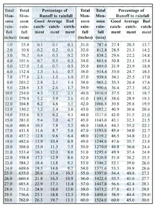
Since there is no appreciable runoff due to the rains in the dry (non-monsoon) period, the monsoon season runoff volume is recommended to be taken as annual yield of the catchment. This table could be used to estimate the monthly yields also in the monsoon season. However, it is to be used with the understanding that the table indicates relationship between cumulative monthly rainfall starting at the beginning of the season and cumulative runoff, i.e. a double mass curve relationship.

(II) Estimating the Runoff Volume from Daily Rainfall

In this method Strange in a most intuitive way recognizes the role of antecedent moisture in modifying the runoff volume due to a rainfall event in a given catchment. Daily rainfall event are considered and three states of antecedent moisture conditions prior to the rainfall event as dry, damp and wet are recognized. The classification of these three states is as follows:

(1) Wetting Process

(a) Transition from Dry to Damp

(i) 6 mm rainfall in the last 1 day (iii) 25 mm in the last 7 days

(ii) 12 mm in the last 3 days (iv) 38 mm in the last 10 days

(b) Transition from Damp to Wet

(i) 8 mm rainfall in the last I day (iii) 25 mm in the last 3 days

(ii) 12 mm in the last 2 days (iv) 38 mm in the last 5 days

Whenever 64 mm rain falls on the previous day or on the same day.

(2) Drying Process

(d) Transition from Wet to Damp

(i) 4 mm rainfall in the last 1 day (iii) 12 mm in the last 4 days

(ii) 6 mm in the last 2 days (iv) 20 mm in the last 5 days

(e) Transition from Damp to Dry

(i) 3 mm rainfall in the last I day (iii) 12 mm in the last 3 days

(ii) 6 mm in the last 3 days (iv) 15 mm in the last 10 days

The percentage daily rainfall that will result in runoff for average (yield producing) catchment is given in Table 19.2(b). For good (yield producing) and bad (yield producing) catchments add or deduct 25% of the yield corresponding to the average catchment.

Table 19.2b.Strange's Table of Runoff Volume from Daily Rainfall

For an Average Catchment(Source: Subramanya, 2008)

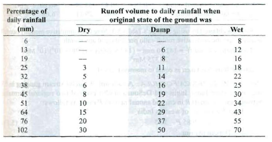
Use of Strange's Tables

Strange's monsoon rainfall-runoff table (Table 19.2a) and (Table 19.2b) for estimating daily runoff corresponding to a daily rainfall event are in use in parts of Karnataka, Andhra Pradesh and Tamil Nadu.

19.1.4 Inglis and Desouza Formula

As a result of careful stream gauging in 53 sites in Western India, Inglis and DeSouza (1929) evolved two regional formulae, between annual runoff R in cm and annual rainfall P in cm as follows:

1.For Ghat regions of western India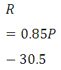
(19.2)

2.For Deccan plateau

(19.3)

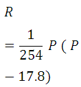
19.1.5 Khosla’s Formula

Khosla (1960) analyzed the rainfall, runoff and temperature data for various catchments in India and USA to arrive at an empirical relationship between runoff and rainfall. The time period is taken as a month. His relationship for monthly runoff is

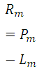(19.4)

and

(19.5)

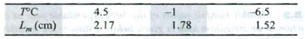
where R_m= monthly runoff in cm and R_m ≥ 0; P_m =monthly rainfall in cm; L_m= monthly losses in cm; T_m= mean monthly temperature of the catchment in °C

For, T_m ≤ the loss may provisionally be assumed as

Annual runoff = ∑ R_m

Khosla’s formula is indirectly based on the water-balance concept and the mean monthly catchment temperature is used to reflect the losses due to evapotranspiration. The formula has been tested on a number of catchments in India and is found to give fairly good results for the annual yield for use in preliminary studies.

19.2 Rational Method

Consider a rainfall of uniform intensity and very long duration occurring over a basin. The runoff rate gradually increases from zero to a constant value as indicated in Fig. 19.1.

Fig. 19.1.Runoff Hydrograph due to Uniform Rainfall.(Source: Subramanya, 2008)

The runoff increases as more and more flow from remote areas of the catchment reach the outlet. Designating the time taken for a drop of water from the farthest part of the catchment to reach the outlet as t_c= time of concentration, it is obvious that if the rainfall continues beyond t_c, the runoff will be constant and at the peak value. The peak value of the runoff is given by

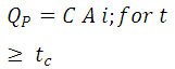(19.6)

WhereC is coefficient of runoff = (runoff/rainfall), A is area of the catchment andi is intensity of rainfall. This is the basic equation of the rational method.

Using the commonly used units, Eq. (19.6) is written for field application as

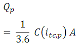(19.7)

WhereQ_p= peak discharge (m³/s); C = coefficient of runoff; (i_tc,p) = the mean intensity of precipitation (mm/h) for a duration equal to t_cand an exceedence probability P; A= drainage area in km². The use of this method to compute Q_prequires three parameters: t_c,(i_tc,p) and C.

19.2.1 Time of Concentration(t_c)

KirpichEquation (1940)

This is the popularly used formula relating the time of concentration of the length of travel and slope of the catchment as

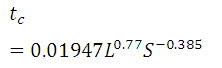(19.8)

Wheret_c is time of concentration (minutes); L is maximum length of travel of water (m) and S is slope of the catchment = ΔH/Lin which ΔH is difference in elevation between the most remote point on the catchment and the outlet.

Rainfall Intensity (i_tc,p)

The rainfall intensity corresponding to a duration and the desired probability of exceedenceP, (i.e. return period T = 1/P) is found from the rainfall-frequency-duration relationship for the given catchment area. This relationship is given as

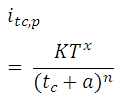(19.9)

WhereK, a, x and n are coefficients, specific to a given area.

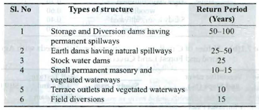
The recommended frequencies for various types of structures used in watershed development projects in India are as below:

Table 19.3. Frequencies for various types of structures in India(Source: Subramanya, 2008)

Runoff coefficient (C)

The coefficient C represents the integrated effect of the catchment losses and hence depends upon the nature of the surface, surface slope and rainfall intensity. Some typical values of C are indicated in Table 19.4 (a and b).

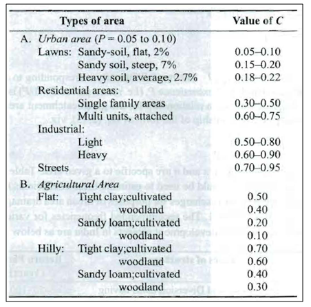
Table 19.4a. Value of the Coefficient C in Eq. (19.7)(Source: Subramanya, 2008)

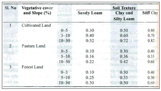
Table 19.4b. Values of C in Rational Formula for Watersheds with

Agricultural and Forest Land Covers(Source: Subramanya, 2008)

Equation (19.7) assumes a homogeneous catchment surface. If however, the catchment is non-homogeneous but can be divided into distinct sub areas each having a different runoff coefficient, then the runoff from each sub area is calculated separately and merged in proper time sequence. In such cases a weighted equivalent runoff coefficient C_eas below is used.

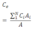(19.10)

Whereis the areal extent of the sub area ihaving a runoff coefficient C, and N is number of sub areas in the catchment.

The rational formula is found to be suitable for peak-flow prediction in small catchment up to 50 km² in area. It finds considerable application in urban drainage designs and in the design of small culverts and bridges.

19.3 Cook’s Method

Cook used a different approach to estimate the runoff from small agricultural areas. In this method, the runoff characteristics of a watershed are examined under four categories:

Relief
Infiltration
Vegetative cover
Surface storage

Based on observations of peak floods from agricultural areas, numerical values have been assigned to the various conditions of above categories by various investigators.

Steps

The sum,Σ W, of the numerical values assigned to the watershed characteristics is obtained.
Runoff curves (relating runoff with drainage area for Σ W values) are then entered with the drainage area and Σ W and the value of peak runoff for a 10 year recurrence interval is obtained.
This peak runoff value is then modified for recurrence interval and geomorphic characteristics by the formula:

Q = P . R . F (19.11)

WhereQ is peak runoff for a specified RI and geomorphic location, P is peak runoff obtained in step 2, R is geomorphic rainfall factor (based on longitude and latitude), F is recurrence interval factor.

Return Period, years	Factor, F
10	1.0
25	1.2
50	1.4

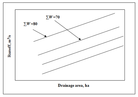
Fig. 19.2.Relationship between drainage area and runoff for a given RI. (Source: Suresh, 2007)

References

Subramanya, K.(2008). Engineering Hydrology.Third Edition, Tata McGraw Hill, 155-162.

Suresh, R. (2007). Soil and Water Conservation Engineering.Second edition, Standard Publishers Distributers, 44-46.