Watershed Planning and Management

Lesson 12 Measurement of Water Yield from Watersheds

12.1.1 Surface Water

Stream gauging in a stream is a technique used to measure the discharge, or the volume of water moving through a channel per unit time. The depth of water in the stream channel, known as a stage or gauge height can be used to determine the discharge in a stream. When used in conjunction with velocity and cross-sectional area measurements, stage height can be related to discharge. If a weir or flume (devices, generally made of concrete, located in a stream channel that have a constant known shape and size) is used, based on the weir or flume shape, mathematical equations can be helpful for velocity measurements. Stream gauging can be done by measuring the stage height and velocity at a series of points in a cross-section of a stream or by constructing a flume or weir and recording stage height. Different methods of measuring stream flow are as below.

12.1.1.1 Stage and Velocity or Velocity-Area Method

Discharge, or the volume of water flowing in a stream over a set interval of time, can be determined with the equation:

Q = AV

where, Q is discharge (volume/unit time - e.g. m³/s, also called cumecs), A is the cross-sectional area of the stream (e.g. m²), and V is the average velocity (e.g. m/s).

Stream water velocity is typically measured using a current meter. Current meters generally consist of a propeller or a horizontal wheel with small, cone-shaped cups attached to it which fill with water and turn the wheel when placed in flowing water. The number of rotations of the propeller or wheel-cup mechanism corresponds with the velocity of the water flowing in the stream. Water flowing within a stream is subject to friction from both the stream bed and the air above the stream. Thus, when taking water velocity measurements, it is conventional to measure flow at 0.6 times the total depth, which typically represents the average flow velocity in the stream. This is achieved by attaching the current meter to a height-calibrated rod. The rod can also be used to measure stream stage height. If a current meter is not available, another technique known as the float method can be used to measure velocity. While less accurate, this method requires limited and easy to obtain equipment. To measure velocity via the float method, one simply measures the time a floating object (such as a piece of wood) takes to travel a measured distance. This is done in a relatively straight channel section length of 30 m. Velocity is then calculated by dividing the distance traveled by the float in observed time.

Velocity also varies within the cross-section of a stream, where stream banks are associated with greater friction, and hence slower moving water. Thus, it is necessary to take velocity measurements along a cross-section of a stream. Since stream channels are rarely straight, it is helpful to measure velocity across an "average" reach of the stream (e.g. average width and depth) with a single channel, a relatively flat stream bed with little vegetation and rocks, and few back-eddies that hinder current meter movement.

Discharge is measured by integrating the area and velocity of each point across the stream; that is, the stream is divided into sections. By multiplying the cross-sectional area (width of section x stage height) by the velocity, one can calculate the discharge for that section of stream. The discharge from each section can be added to determine the total discharge of water from the stream.

Discharge and stage height are often found to be empirically related and this relationship can be elucidated using a rating curve. A rating curve is constructed by graphing several manually derived discharge measurements with a corresponding stage height. A best-fit curve is fit to these data points and the equation of the line corresponds to the relationship between stage and discharge. The greater the number of measurements, the more reliable the rating curve will be to determine discharge based on stage data.

12.1.1.2 Measuring Discharge Using a Weir

Discharge in small streams can be conveniently measured using a weir. A weir is a small dam with a spillway of a specific shape, usually made of erosion-resistant material such as concrete. Two common weir shapes are a 90° V-notch or a simple rectangular cutout. This method for measuring discharge involves creating a dam just downstream of the weir. This dam impounds in the weir, resulting in a more or less consistent stage height (e.g. a pool of more stagnant water without complications determining height due to waves or ripples). Using the height of water over the weir crust, discharge is determined using empirically-derived equations, as below.

Rectangular Weir (Fig. 12.1):

Q = 3.33 (L-0.2H) H^3/2, in feet;

Q= 1.84 (L-0.2H) H^2/3, in meters.

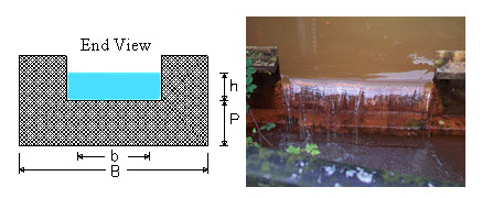
Fig. 12.1. Rectangular Weir.

(Source: http://www.ussi.co.uk/Weirs_and_Flumes.html)

90° V-notch weir (Fig. 12.2):

Q = 2.5H^5/2, in feet;

Q = 1.379H^5/2, in meters

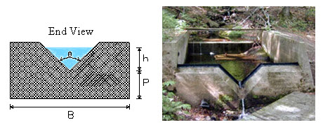
Fig. 12.2. 90° V-notch Weir.

(Source: http://www.lmnoeng.com/Weirs/vweir.htm)

Q represents discharge (ft³/s or m³/s), L is the length of the weir crest (ft or m), and H is the height of the water in the backwaters/weir (ft or m). These equations negate the need for measuring point velocities and are generally more reliable since the concrete construction of the weir resists change in channel shape, which is a confounding factor when using the velocity-area method to determine discharge.

12.1.1.3 Discharge Measurement by Tracer Methods

Velocity-Area Tracer Discharge Equation: The discharge using velocity-area method is computed by –

Q=AL/T        

Where, Q = discharge in cubic feet per second (ft³/s), A = average cross-sectional area of reach length in square feet (ft²), L = reach length between detection stations in feet (ft), T = recorded time required for the tracer solution to travel between the detection stations at each end of the measurement reach in seconds (s)

Tracer-Dilution Discharge Equation: The dilution method equation for discharge is –

QC₀+qC₁ = (Q+q) C₂

Q = q (C₁-C₂)/(C₂-C₀)

Where, C₀ = the natural or background concentration of the tracer of the flow, C₁ = the concentration of the strong injected tracer solution, C₂ = the concentration of tracer after full mixing at the sampling station, including the background concentration of the stream, Q = the discharge being measured, q = the discharge of the strong solution injected into the flow.

The discharge of the channel flow, Q, is measured by determining C₀, C₁, C₂, and the injection rate, q. Only the final plateau value or C₂, the downstream concentration, must be recorded rather than a complete record of the passing cloud that is needed with the salt-velocity-area method.

12.1.2 Measurement of Ground Water Yield

12.1.2.1 Seepage Meters for Measuring Groundwater

Seepage meters (Fig. 12.3) measure the quantity of water moving into or out of the river through the streambed sediments. Such measurements help quantify ground water/surface water interchange. Seepage meter methods determine the variability of ground-water discharge and recharge at specific locations in the streambed which provides local-scale stream bed heterogeneity. This method uses an open-ended drum pushed into the streambed to measures the amount of water that is lost or gained in the bag connected to the seepage meter over time. Seepage from the bottom sediment is collected in a plastic bag to estimate specific discharge q (m/s).

q = Q/A

Where, Q (m³/s) is the flow rate and A (m²) is the area covered by the seepage meter.

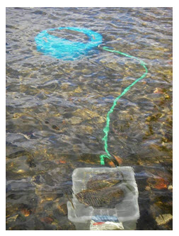
Fig. 12.3. Seepage Meter.

(Source:  http://astro.temple.edu/~ltoran/docs/gw_sw.htm)

Working of Seepage Meter

The basic concept of a seepage meter is to enclose and isolate an area of the sediment–surface water interface with a cylinder that is open at its base and vented at the top to a plastic collection bag. The change in the volume of water in the collection bag over a measured time interval is used to determine the direction and rate of flow between surface water and groundwater. A gain in water volume in the collection bag indicates that flow is occurring from groundwater to surface water, while a loss in water volume indicates that flow is occurring from surface water to groundwater. Seepage meters have an advantage over other methods of measuring groundwater–surface water exchange since flow measurements can be made without measurement of the hydraulic conductivity of the sediment. Seepage meters are particularly useful when many measurements are needed in order to characterize groundwater–surface water exchange in different segments of a water body.

12.1.2.2 Mini-piezometers

Mini-piezometers are simple instruments for measuring the direction of water flow between groundwater and a surface water body such as a lake or stream (Fig. 12.4). Often temporarily installed, mini-piezometers are essentially scaled-down versions of piezometers, which are routinely used to make groundwater level measurements. When combined with surface water level measurements, this can be used to determine the direction of water flow. When flow measurements from seepage meters are combined with hydraulic head measurements from mini-piezometers, the hydraulic conductivity of the bottom sediment can be calculated.

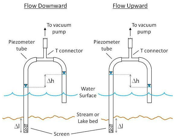
Fig. 12.4. Flow Downward (Left) Indicated by the Surface Water Level > Groundwater Level and Flow Upward (Right) Indicated by the Surface Water Level < Groundwater Level. (Source: Christopher, 2013)

12.1.3 Measurement of Lateral Flow or Interflow

Interflow is the portion of the stream flow contributed by infiltrated water that moves laterally in the subsurface until it reaches a channel. Interflow is a slower process than surface runoff. Components of interflow are quick interflow; which contributes to direct runoff; and delayed interflow, which contributes to base flow (Fig. 12.5). Interflow velocities are measured with different measuring devices (TDR-waveguides, FD-probes, geoelectrics, changes of conductivity in antecedent water courses, and others) for the assessment of bandwidths of lateral and vertical conductivity during and after long-lasting rainfall.

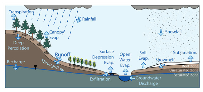
Fig. 2.5. Hydrological Cycle showing Runoff Processes.

(Source: http://hydrogeology.glg.msu.edu/research/active/modeling-and-monitoring-hydrologic-processes-in-large-watersheds)

Infiltrated water is initially referred as the Upper Zone Storage (UZS). Water within this layer percolates downward or is exfiltrated to nearby water courses, and is called interflow. Interflow is represented by a simple storage-discharge relation;

DUZ = REC * (UZS-RETN) *Si

where: DUZ = the depth of upper zone storage released as interflow in mm, REC = a dimensionless coefficient (optimized), UZS = water accumulation in the upper zone region in mm, RETN = retention and Si = internal slope (land surface slope). REC is a coefficient, which cannot be predicted, and is therefore estimated through optimization. Values of REC are expressed as the depletion fraction per hour of the Upper Zone storage and range from 0.001 to 0.005 i.e., from 0.1 to 0.5 percent of the water stored in the upper zone is drained off each hour. DUZ is calculated simultaneously with Upper Zone to Lower Zone drainage.

12.1.4 Measurement of Seepage Flow

Seepage occurs in all three dimensions and Darcy’s law is applicable when flow of water is in one direction. Solution for 3D problems is complicated and needs advanced mathematical calculations. In many cases, 3D problems are simplified to 2D and seepage flow is calculated accordingly using Laplace Equation.

Laplace graphical solution (Flow Net) requires 2 families of curves that meet at right angle. One is called flow line and the other is called equi-potential line. The network of these lines is called “Flow Net” (Fig. 12.6). Properties of flow net are; same flow quantity through each flow channel and same head drop between each adjacent pair of equi-potential lines (except for partial drop).

Fig. 12.6. Example of Flow Net Beneath a Dam Structure.

(Source: Fung, 2008)

12.1.5 Water from Outside Watershed Boundary

The flowing water above or below the ground does not follow any local and political boundaries. However, it moves with natural gradient. Due to this property, water flows to and from neighboring watersheds. Accurate measurement of this incoming or outgoing water from the watershed, in consideration, is quite difficult. To quantify and assess this water, modeling serves as a better tool when using the process and interaction information characteristics of the watersheds.  

12.2 Modeling and Assessment of Water Resources in Watersheds

Measurement of water yield in a watershed is a time taking, tedious and difficult process. It involves several instrumental as well as human error possibilities. To reduce these negative aspects and to get quick information, modeling is often used as tool to assess the water yield of a watershed. The detail of modeling of watershed water resources is discussed as below.

12.2.1 Purpose and Scope of Watershed Modeling

A watershed model simulates hydrologic processes in a more holistic approach compared to many other models which primarily focus on individual processes or multiple processes at relatively small-or field-scale without full incorporation of a watershed area. Watershed-scale modeling has emerged as an important scientific research and management tool, particularly in efforts to understand and control water pollution. Watershed modeling involves a holistic approach that involves not only examining surface hydrology, groundwater hydrology, or their interface as whole systems, but attempting to imitate the three regions as one system. One limitation is the availability of precipitation, flow, land cover, etc. data for the entire region. Another consideration is the limited understanding of the interactions between smaller hydrologic entities.

12.2.2 Models Used for Watershed Modeling

Watershed models can be grouped into various categories based upon the modeling approaches used. The primary features for distinguishing watershed-scale modeling approaches include the nature of the employed algorithms (empirical, conceptual, or physically-based), whether a stochastic or deterministic approach is used for model input or parameter specification, and whether the spatial representation is lumped or distributed. Various watershed models developed and used for assessing the watershed water yield can be categorized based on their characteristics, and time and spatial scale of use as below.

12.2.2.1 Based on Nature of Input and Uncertainty

Watershed models can be categorized as deterministic or stochastic depending on the techniques involved in the modeling process. Deterministic models are mathematical models in which outcomes are obtained through known relationships among states and events. Stochastic models will have most, if not all, of their inputs or parameters represented by statistical distributions which determine a range of outputs.

12.2.2.2 Based on Nature of the Algorithms

Physically-based models are based on the understanding of the physics associated with the hydrological processes which control catchment response and utilize physically based equations to describe these processes. Empirical models consist of functions used to approximate or fit available data. Such models span to a range of complexity, from simple regression models to hydro informatics based models which utilize Artificial Neural Networks (ANNs), Fuzzy Logic, Genetic, and other algorithms.

12.2.2.3 Based on Nature of Spatial Representation

Watershed-scale models can further be categorized on a spatial basis as lumped, semi-distributed, or distributed models. The lumped modeling approach considers a watershed as a single unit for computations and the watershed parameters and variables are averaged over this unit. Compared to lumped models, semi-distributed and distributed models account for the spatial variability of hydrologic processes, input, boundary conditions, and watershed characteristics. For semi-distributed models, the aforementioned quantities are partially allowed to vary in space by dividing the basin into a number of smaller sub-basins, which in turn are treated as a single unit. These models describe mathematically the relation between rainfall and surface runoff without describing the physical process by which they are related eg. Unit Hydrograph approach. Spatial heterogeneity in distributed models is represented with a resolution typically defined by the modeler.

12.2.2.4 Based on Type of Storm Event

Watershed-scale models can be further subdivided into event-based or continuous-process models. Event-based models simulate individual precipitation-runoff events with a focus on infiltration and surface runoff, while continuous process models explicitly account for all runoff components while considering soil moisture redistribution between storm events.

Keywords: Surface Water, Groundwater, Lateral Flow, Seepage, Watershed Modelling.

References

• http://www.ussi.co.uk/Weirs_and_Flumes.html. Last seen: 29^th September 2013

• http://www.lmnoeng.com/Weirs/vweir.htm. Last seen: 29^th September 2013

• http://astro.temple.edu/~ltoran/docs/gw_sw.htm. Last seen: 29^th September 2013

• http://hydrogeology.glg.msu.edu/research/active/modeling-and-monitoring-hydrologic-processes-in-large-watersheds. Last seen: 29^th September 2013

• Christopher J. M, 2013. University of Florida. URL:http://edis.ifas.ufl.edu/LyraEDISServlet?command=getImageDetail&image_soid=FIGURE%201&document_soid=AE454&document_version=39770. Last accessed: 29^th September 2013

• Fung F. C., 2008. An Approach to the Mechanics of Fluids. URL: http://www.fcfung2000.com/moffiles/mofflown.htm. Last seen: 29^th September 2013

Suggested Readings

• McMahon, T. A., & Mein, R. G. (1986). River and reservoir yield. Littleton, Colorado, USA: Water resources publications.

• Ratnayaka, D. D., Brandt, M. J., & Johnson, M. (2009). Water Supply. Butterworth-Heinemann.