Watershed Planning and Management

Lesson 18 Estimation and Modeling of Sediment Yield

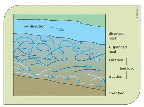
Fig. 18.1. Illustration of Different Types of Sediment Loads.

(Source: http://riverrestoration.wikispaces.com/Sediment+transport+models)

1.        Dissolved Load: Dissolved load is material that has gone into solution and is part of the fluid moving through the channel. Since it is dissolved, it does not depend on forces in the flow to keep it in the water column. The amount of material in solution depends on supply of a solute and the saturation point for the fluid. For example, in limestone areas, calcium carbonate may be at saturation level in river water and the dissolved load may be close to the total sediment load of the river. In contrast, rivers draining through insoluble rocks, such as in granitic terrains, may be well below saturation levels for most elements and dissolved load may be relatively small. The dissolved load is also very sensitive to water temperature and due to this reason, tropical rivers carry larger dissolved loads than those in temperate environments. Total dissolved-material transport, Q_s(d) (kg/s), depends on the dissolved load concentration C₀ (kg/m³), and the stream discharge, Q (m³/s)

Q_s(d) = C₀Q

2.        Suspended Load: Suspended load comprises sand+silt+clay sized particles that are held in suspension because of the turbulence of the water. The suspended load is further divided into the wash load, which is generally considered to be the silt+clay sized material (< 62 μm particle diameter) and is often referred to as “fine-grained sediment”. Suspended load moves at the same velocity as the flow. The upward currents must equal or exceed the particle fall-velocity (Fig. 18.2) for suspended sediment load to be sustained.

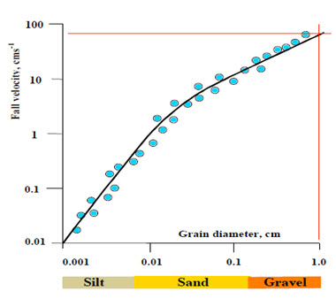
Fig. 18.2. Fall Velocity in Relation to Diameter of a Spherical Grain of Quartz.

(Source:http://www.sfu.ca/~hickin/RIVERS/Rivers4(Sediment%20transport).pdf)

3.        Intermittently Suspension or Saltation Load: Saltation load is a term used by sedimentologists to describe material that is transitional between bed load and suspended load. Saltation means “bouncing” and refers to particles that are light enough to be picked off the river bed by turbulence but too heavy to remain in suspension and, therefore, sink back to the river bed. These are particles that bounce along the channel, partly supported by the turbulence in the flow and partly by the bed. They follow a distinctively asymmetric trajectory.

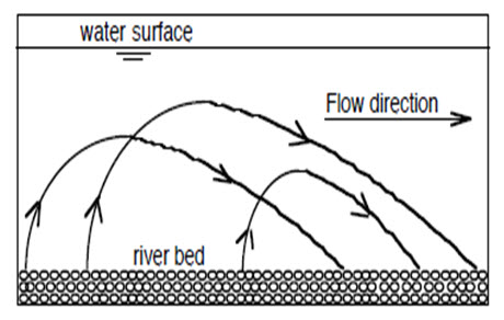
Fig. 18.3. The Trajectory of Sediment Saltation (Intermittently Suspended)

Grains Moving in the Flow. (Source:http://www.sfu.ca/~hickin/RIVERS/Rivers4(Sediment%20transport).pdf)

4.        Wash Load: Analysis of suspended load and the corresponding bed materials of various streams for their size analysis have shown that the suspended load can be divided into two parts depending on the sizes of material in suspension vis-à-vis the size analysis of the bed material. One part of the suspended load is composed of these sizes of sediment found in abundance in the bed. The second part of the load is composed of those fine sizes not available in appreciable quantities in the bed. These particles, termed as the wash load, actually originate from the channel bank and the upslope area. Wash load grains tend to be very small (clays and silts) and, hence have a very small settling velocity. Once introduced into the channel, wash-load grains are kept in suspension by the flow turbulence and essentially pass straight through the stream with negligible deposition or interaction with the bed.

5.        Bed Load: Bed load is the clastic (particulate) material that moves through the channel fully supported by the channel bed itself. These materials, mainly sand and gravel, are kept in motion (rolling and sliding) by the shear stress acting at the boundary. A distinction is often made between the bed-material load and the bed load. Bed-material load is that part of the sediment load found in appreciable quantities in the bed (generally > 0.062 mm in diameter) and is collected in a bed-load sampler. It includes particles that slide and roll along the bed (in bed-load transport) but also those near the bed transported in saltation or suspension. Bed load, strictly defined, is just that component of the moving sediment that is supported by the bed (and not by the flow). That is, the term “bed load” refers to a mode of transport and not to a source.

After successful measurements of different sediment loads flowing along with river/channel water, the estimation of watershed sediment load is performed to find out total soil/sediment loss from the watershed. In this process, bed load and suspended load are separately estimated for the desired time (second, day, month, year) and then summed up to find out total sediment load from the watershed. The methods of estimating these loads of watershed are discussed as below. 

Suspended Load

The amount of suspended load transported in a day (for an example here) is given by:

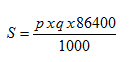
Where, S  = amount of material transported in tonnes/day;  = amount of material in 1 cu.m. of water in kg;  = rate of stream flow in m³/s.

Bed Load

The bed load which is collected in the sampler is dried and weight. The dry weight when divided by time taken for the measurement and the width of the sampler, gives the rate of bed load movement per unit width of the river bed per unit time at the point of measurement. For design purpose bed load is generally taken as certain percentage of suspended load as:

Table 18.1. Maddock's classification for estimation of the bedload (Maddock, 1975)

Concentration of Suspended Load (ppm)	Type of Material forming the Stream Channel	Texture of Suspended Material	% of Measured Suspended Load that could be taken as Bed Load
Less than 1000	Sand	Similar to bed material	25 to 150
Less than 1000	Gravel, rock or consolidate clay	Small amount of sand	5 to 12
1000 to 7500	Sand	Similar to bed material	10 to 35
1000 to 7500	Gravel, rock or consolidate clay	25% sand or less	5 to 15
Over 7500	Sand	Similar to bed material	5 to 15
Over 7500	Gravel, rock or consolidate clay	25%  sand or less	2 to 8

(Source: http://www.fao.org/docrep/t0848e/t0848e-10.htm)

Once the bed and suspended loads are calculated the total sediment load for each day or for any required period can be easily calculated.

18.2 Modeling of Sediment Yield from Watersheds

Modeling is a useful tool for erosion scenario assessment that enables the adequate selection of erosion control measures (Moehansyah et al, 2004). Sediment models are to link the on-site rates of erosion and soil loss within the watershed to the outlet sediment yield. Erosion and sediment yield can be predicted by using two main types of models- empirical and physically based models. The first group is based on the identification of relationships between different watershed property parameters with the sediment generated from watershed when a robust data base exists. These relationships must be statistically significant. Physically based models consist of the description of processes (involved in sediment initiation, generation and transport etc.) with the help of mathematical equations dealing with the laws of conservation of energy and mass (Morgan, 2005). They integrate both the detachment and transport processes for upstream locations and channels.

The first developed and widely used empirical model for sediment yield estimation is USLE (Universal Soil Loss Equation). Due to some practical limitation it has been modified MUSLE (Modified Universal Soil Loss Equation). The description about these empirical models is as below.

18.2.1 Universal Soil Loss Equation (USLE): The Universal Soil Loss Equation (USLE) predicts the long term average annual rate of erosion on a field slope based on rainfall pattern, soil type, topography, crop system and management practices. USLE only predicts the amount of soil loss that results from sheet or rill erosion on a single slope and does not account for additional soil losses that might occur from gully, wind or tillage erosion. This erosion model was created for use in selected cropping and management systems, but is also applicable to non-agricultural conditions such as construction sites. The USLE can be used to compare soil losses from a particular field with a specific crop and management system to "tolerable soil loss" rates. Alternative management and crop systems may also be evaluated to determine the adequacy of conservation measures in farm planning.

Five major factors are used to calculate the soil loss for a given site. Each factor is the numerical estimate of a specific condition that affects (represent) the severity of soil erosion at a particular location. The erosion values reflected by these factors can vary considerably due to varying weather conditions. Therefore, the values obtained from the USLE more accurately represent long-term averages. The USLE is expressed as:

A = R × K × L × S × C × P                                                                               

Where, A = Gross amount of soil erosion (tonnes.ha^-1.yr^-1.) and represents the potential long term average annual soil loss in tons per hectare per year. R = Rainfall factor related to rainfall-runoff erosion (MJ.mm.ha ^-1h ^-1); K = Soil erodibility factor related to soil erosion (t.ha.h.MJ^-1 mm^-1); L = Slope length factor (dimensionless); S = Slope steepness factor (dimensionless); C = Factor related to cover management (dimensionless); P = Factor representing the supporting practices applied (dimensionless)

Procedure for Using the USLE

1. Determine the R Factor

2. Based on the soil texture, determine the K value. If there is more than one soil type in a field and the soil textures are not very different, use the soil type that represents the majority of the field. Repeat for other soil types as necessary

3. Divide the field into sections of uniform slope gradient and length. Assign an L value to each section

4. Choose the crop type factor and tillage method factor for the crop to be grown. Multiply these two factors together to obtain the C factor

5. Select the P factor based on the support practice used

6. Multiply the 5 factors together to obtain the soil loss per hectare (acre)

18.2.2 Modified USLE: The MUSLE equation is applicable to the points, where overland flow enters the streams and then all those points are summed up to give the total amount of sediment delivered to the stream network within a watershed. Williams (1975) developed the MUSLE by replacing the rainfall energy factor in the USLE with a runoff energy factor. In general, MUSLE is expressed as follows (Williams, 1975):

Where, Y is the sediment yield to the stream network in metric tons, Q is the runoff volume from a given rainfall event in m³, q_p is the peak flow rate in m³/sec., K is the soil erodibility factor, LS is the slope length and gradient factor, C is the cover management factor and can be derived from land cover data, and P is the erosion control practice factor which is a field specific value. The Q, q_p, and LS parameters can be derived from Digital Elevation Model (DEM), land cover, soil, and rainfall data.

18.3 Watershed Hydrologic Models used in Sediment Yield Estimation

 Sediment transport models are being developed to assist state and local resource agencies for the purpose of developing appropriate management plans to reduce/control sedimentation problems in the watersheds. Use of models in identifying areas with high sediment yield that can be of dredging concern.  Controlling sediment loads requires knowledge and quantitative assessment of soil erosion and the sediment transport process. A number of factors such as drainage area size, basin slope, climate, land use/land cover affect sediment delivery processes.

Under hydrologic models for sediment yield estimation, models can be called parametric, deterministic, or physically based models. These models are developed based on the fundamental hydrological and sedimentological processes. They may provide detailed temporal and spatial simulation but usually require extensive data input. Below are the few models and their parameters required to estimate sediments from the watersheds used extensively for the purpose.

1. AGNPS (Agricultural Non Point Source Pollution, 1985): It requires 22 parameters for each grid cell (area unit) and there is a limitation for the number of cells in running the model.

2. CREAMS (Chemicals, Runoff, and Erosion from Agricultural Management Systems, 1980):  It evaluates non point source pollution (sediment and agro-chemicals) from field plots.

3. SPUR (Simulation of Production and Utilization of Rangelands, 1983): The process oriented model used to replace the USLE for routine assessment of watershed characteristics.

4. Hydrologic models such as GSSHA (Gridded Surface/Subsurface Hydrologic Analysis), SWAT (Soil and Water Assessment Tool): They require even larger quantity of input data. Hourly/daily input values of meteorological and radiation variables are required for continuous simulations.

5. Other models include

   1. EUROSEM (European Soil Erosion Model)

   2. KINEROS (Kinematic runoff and erosion model)

   3. LISEM (LImburg Soil Erosion Model)

   4. WEPP (Water Erosion Prediction Project)

   5. ANSWERS (Areal Non point Source Watershed Environment Response Simulation)

   6. GLEAMS (Groundwater Loading Effects of Agricultural Management Systems)

   7. EPIC

Keywords: Sediment Load, Sediment Yield, Sediment Yield Modeling, Universal Soil Loss Equation

References

• http://riverrestoration.wikispaces.com/Sediment+transport+models

• http://www.sfu.ca/~hickin/RIVERS/Rivers4(Sediment%20transport).pdf

• Maddock T. (1975). Table 3.2 in Sediment Engineering, V.A. Vanoni (ed.). ASCE, New York.

Suggested Readings

• Murthy V.V.N. (1985). Land and Water Management Engineering, Kalyani publishers, pp 559- 564.

• Suresh R. (1993). Soil and water conservation eng., Standard Publishers Distributors, New Delhi, chapter 19.

• Madsen, O.S. (1993).  Sediment transport on the shelf. Short Course attached to 25^th International Conference on Coastal Engineering, Orlando, USA, 1996

• Hickin, E.J. (1989). Contemporary Squamish River sediment flux to Howe Sound, British Columbia. Canadian Journal of Earth Sciences, 26: 1953-1963

• www.omafra.gov.on.ca/english/engineer/facts/00-001.htm

• ISO 1985 Liquid Flow in Open Channels - Sediment in Streams and Canals – Determination of Concentration, Particle Size and Relative Density. International Standard ISO 4365, International Organization for Standardization, Geneva.

• NRCS. (2004). National Engineering Handbook. Part 630 Hydrology, 210-VI-NEH-630.10 US Department of Agriculture: Washington DC, p. 10-1 to 10-5.