System Engineering

LESSON 2. Graphical Method I

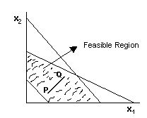
2.2 Feasible Region

It is the collection of all feasible solutions. In the following figure, the shaded area represents the feasible region.

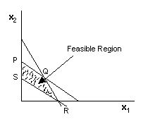
2.3 Convex Set

A region or a set R is convex, if for any two points on the set R, the segment connecting those points lies entirely in R. In other words, it is a collection of points such that for any two points on the set, the line joining the points belongs to the set. In the following figure, the line joining P and Q belongs entirely in R.

                                   

Thus, the collection of feasible solutions in a linear programming problem form a convex set

2.4 Graphical Method - Algorithm

1. Formulate the mathematical model of the given linear programming problem.

2. Treat inequalities as equalities and then draw the lines corresponding to each equation and non-negativity restrictions.

3. Locate the end points (corner points) on the feasible region.

4. Determine the value of the objective function corresponding to the end points determined in step 3.

5. Find out the optimal value of the objective function.

2.5 Redundant Constraint

It is a constraint that does not affect the feasible region.

Consider the linear programming problem:

                 Maximize 1170 x₁ + 1110x₂

subject to

9x₁ + 5x₂≥ 500

7x₁ + 9x₂ ≥ 300

5x₁ + 3x₂≤ 1500

7x₁ + 9x₂ ≤1900

2x₁ + 4x₂ ≤ 1000

      x₁, x₂ ≥ 0

The feasible region is indicated in the following figure:

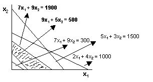
The critical region has been formed by the two constraints.

9x₁ + 5x₂ ≥ 500
7x₁ + 9x₂ ≤ 1900

x₁, x₂ ≥ 0

The remaining three constraints are not affecting the feasible region in any manner. Such constraints are called redundant constraints.

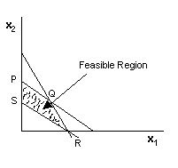
2.6 Extreme Point

Extreme points are referred to as vertices or corner points. In the following figure, P, Q, R and S are extreme points.

Example 1.

Maximize z = 18x₁ + 16x₂

subject to

15x₁ + 25x₂ ≤375
24x₁ + 11x₂ ≤ 264

x₁, x₂ ≥ 0

Solution:

If only x₁ and no x₂ is produced, the maximum value of x₁ is 375/15 = 25. If only x₂ and no x₁ is produced, the maximum value of x₂ is 375/25 = 15. A line drawn between these two points (25, 0) & (0, 15), represents the constraint factor 15x₁ + 25x₂≤ 375. Any point which lies on or below this line will satisfy this inequality and the solution will be somewhere in the region bounded by it.

Similarly, the line for the second constraint 24x₁ + 11x₂≤ 264 can be drawn. The polygon oabc represents the region of values for x₁ & x₂ that satisfy all the constraints. This polygon is called the solution set.

The solution to this simple problem is exhibited graphically below.

 

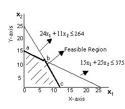
The end points (corner points) of the shaded area are (0,0), (11,0), (5.7, 11.58) and (0,15). The values of the objective function at these points are 0, 198, 288 (approx.) and 240. Out of these four values, 288 is maximum.

The optimal solution is at the extreme point b, where x₁ = 5.7 & x₂ = 11.58, and z = 288.

Example 2

Maximize z = 6x₁ - 2x₂

subject to

2x₁ - x₂ ≤ 2
x₁ ≤ 3

x₁, x₂ ≥ 0

Solution.

First, we draw the line 2x₁ - x₂ ≤ 2, which passes through the points (1, 0) & (0, -2). Any point which lies on or below this line will satisfy this inequality and the solution will be somewhere in the region bounded by it.

Similarly, the line for the second constraint x₁ ≤ 3 is drawn. Thus, the optimal solution lies at one of the corner points of the dark shaded portion bounded by these straight lines.

                                

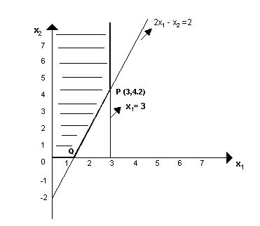
Optimal solution is x₁ = 3, x₂ = 4.2, and the maximum value of z is 9.6.