Drainage Engg.2(1+1)

Lesson 7 Unsteady-State Flow to Drains

7.2  Unsteady-State Drainage Equations

7.2.1   Glover-Dumm Equation

In the case of unsteady/transient flow, the flow is not constant, rather it changes with time as water is stored in or released from the soil. The change in storage is reflected either in a rise or a fall of the water table. The Dupuit-Forchheimer approach is used to derive a differential equation of unsteady flow in the waterlogged soil. Let’s consider a soil column which is bounded by the water table at the top and by an impervious layer at the bottom. If there is no recharge to the groundwater, the change in storage in the soil profile is given as (Fig. 7.1):

 

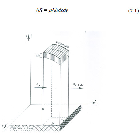
Fig. 7.1. Change in storage in a soil column under a falling water table. (Source: Ritzema, 1994)

Where, DS = change in water storage per unit surface area over a given time [L], m = drainable porosity (dimensionless), and Dh = change in the water table over a given time [L].

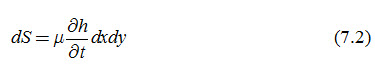
Equation (7.1) can be written as follows if the change in storage is considered over an infinitely small period of time (dt):

 

From the continuity principle, the net inflow or outflow in x-and y-directions is equal to the change in storage. Therefore, using the Darcy’s law the differential form of the two dimensional continuity equation for a homogeneous and isotropic soil profile can be written as:

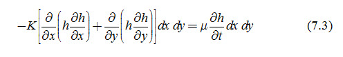
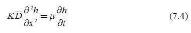
Equation (7.3) is known as the Boussinesq equation which describes the position of the water table under unsteady recharge. It is a non-linear equation, which can be linearized by assuming that initial saturated thickness of the water transmitting layer is (D) large compared to the changes in the water table. Hence, h can be taken as a constant  (average thickness of the water-transmitting layer). Further, in drainage, we deal with only one dimensional flow and hence, Eqn. (7.3) reduces to:

Dumm (1954) used this differential equation to describe the fall of the water table after it had risen instantaneously to a height h₀ above the drain level (Fig. 7.2). His solution, which is based on a formula developed by Glover, describes the lowering of an initially horizontal water table as a function of time, place, drain spacing, and soil properties. It is expressed as follows:

 

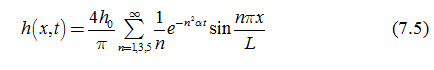
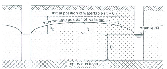
Fig. 7.2. Boundary conditions for the Glover-Dumm equation with an initially horizontal water table. (Source: Ritzema, 1994)

Where,

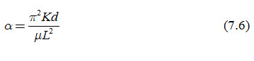
h(x, t) = height of the water table at distance x at time t [L], h₀ = initial height of the water table at t = 0 [L], a = reaction factor [T^-1], K = hydraulic conductivity of the soil layer [L/T], d = equivalent depth of the soil layer below the drain level [L], m = drainable porosity of the soil layer (dimensionless), L = drain spacing [L], and t = time for water table to drop after the instantaneous rise of the water table [T].

The height of the water table at the mid spacing of the drains can be obtained by substituting x = ½ L into Eqn. (7.5) as:

 

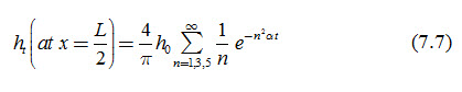
Where, h_t is the height of the water table at the mid-spacing of the drains at t>0 [L].

If at>0.2, the second and subsequent terms of Eqn. (7.7) become small, and hence they can be neglected. Hence, Eqn. (7.7) reduces to:

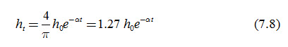
If the initial water table has the shape of a fourth-degree parabola (not horizontal), Eqn. (7.8) becomes (Dumm, 1960):

Now, the substitution of Eqn. (7.6) into Eqn. (7.9) yields an expression for the drain spacing [L] as follows:

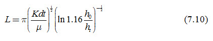
Equation (7.10) is called Glover-Dumm drainage formula, which is recommended for design purposes as illustrated by an example presented later on in this lesson.

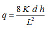
Moreover, the drain discharge per unit surface area at any time (t) can be obtained from the Darcy’s law as:

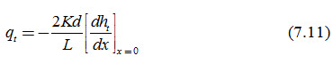
Where, q_t is the drain discharge per unit surface area at t>70 (m/day), and the remaining symbols have the same meaning as defined earlier.

Differentiating Eqn. (7.5) with respect to x as well as neglecting all the terms n>1, substituting x = 0, and combining with Eqn. (7.11) we obtain:

Equation (7.12) can also be written in terms of h_t by substituting Eqn. (7.8). That is,

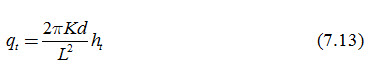
Eqn. (7.13) is similar to the Hooghoudt Equation describing the flow below the drain level, except that the factor 8 is replaced with 2p. Note that for the 4^th degree parabola, 2p becomes 6.89. It can be seen that the drain discharge (q_t) is directly related to the depth of the water table (h_t). This is important when the data from an experimental field are being analyzed, for example, to determine reaction factor (a).

The original Glover-Dumm Equation is based on horizontal flow only and hence it ignores the radial resistance resulting from the convergence of the flow lines near the drains not reaching the impervious layer. However, similar to the steady-state approach, by introducing the Hooghoudt’s concept of the equivalent depth (d) into Eqns. (7.6) and (7.10), the extra resistance caused by the converging flow towards the drains is taken into account by the Glover-Dumm Equation.

7.2.2   De Zeeuw-Hellinga Equation

To simulate the drain discharge over a time period with a non-uniform distribution of recharge, the time period is divided into time intervals of equal length during which recharge (R) is assumed to be constant. The length of the time interval should be such that changes occurring during the time interval could be described sufficiently accurately by the existing steady-state drainage equations, using as input average rates during the interval. This requirement can generally be fulfilled by adopting time intervals (Dt) of length 1 day. De Zeeuw and Hellinga (1958) found that, if the recharge (R) in each time period is assumed to be constant, the change in drain discharge (q) is proportional to the excess recharge (R - q), which is mathematically expressed as:

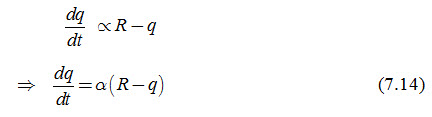
Where, a is the proportionality constant and is known as ‘reaction factor’. Integration of Eqn. (7.14) between the limits t = t; q = q_t and t = t-1; q_t-1 yields:

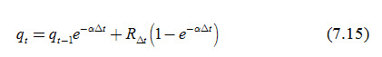
Where, Dt = t – (t - 1), the time interval over which the recharge R_Dt is assumed to be constant (i.e., R_Dt is the mean value of R during the time interval t-1 to t).

We can simulate the depth of the water table by considering the simplified Hooghoudt Equation, which neglects the flow above the drain level and is given as:

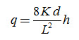
The above equation shows the linear relationship between q and h. By using Eqn. (7.6), we can replace the quotient  of simplified Hooghoudt’s Equation with . Thus, we have:

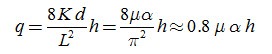
Substituting the latter into Eqn. (7.15) yields:

Equations (7.15) and (7.16) are called De Zeeuw-Hellinga Equations, which can be used to simulate drain discharge and water table fluctuations on the basis of historical water records, provided that the value of the reaction factor (a) is known.

7.2.3 Reaction Factor (a)

The reaction factor  is a direct index of the intensity with which the drain discharge responds to changes in the recharge. According to Smedema and Rycroft (1983), the values of reaction factor generally vary from a = 0.1–0.3 for land with a slow response (low KD values, wide drain spacing, high drainable pore space) to a = 2.0–5.0 for rapidly responsive land (high KD value, narrow drain spacing, low drainable pore space). It may be calculated using Eqn. (7.6) if the values of KD, L and m are known. However, since the m-value is generally difficult to determine, best estimates of a are obtained by observing the actual response of a drainage system in the field (Smedema and Rycroft, 1983). From Eqns. (7.15) and (7.16), it follows that in periods during which there is no recharge (R = 0), the reaction factor (a) can be expressed as follows (Smedema and Rycroft, 1983):

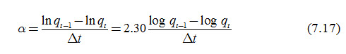
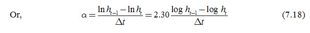
Observed q_t or h_t values can be plotted on the log normal paper. If the system obeys the assumptions underlying the basic equations, the observed values more or less fit to a straight line with a slope equal to a. Observations are best made during periods of low evaporation shortly after the end of a few good rainy days when the recharge to groundwater has ceased and the water table starts receding (the recession sections of the water table or drainflow versus time graphs can be used to estimate a).

7.2.4 Remarks on Unsteady-State Drainage Equations

At first sight, the unsteady-state approach offers major advantages compared to the steady-state approach, but various assumptions restrict the use of the unsteady-state equations. Firstly, both the Glover-Dumm and the De Zeeuw-Hellinga equations can only be applied in soil with a homogeneous profile. Secondly, the flow in the region above the drains is not taken into account. When the depth of the water table above drain level (h) is large compared to the depth of the impervious layer (D), an error may be introduced. However, the biggest restriction is the introduction of drainable pore space into the equations. Besides the fact that this soil property is very difficult to measure, it also varies spatially. Therefore, introducing a constant value for the drainable pore space could result in considerable errors. As a result, the unsteady-state equations are hardly ever used directly in the design of subsurface drainage systems. Instead, it is used in combination with steady-state equations. The benefits of this combined approach are discussed in Section 7.4. Nevertheless, unsteady-state equations are very useful tools when the goal is to study temporal variation of the parameters such as the water table depth or elevation and the drain discharge due to rainfall or irrigation.

7.3  Application of Unsteady-State Drainage Equations

Like the steady-state equations, the unsteady-state equations require data on soil properties and agriculture and technical design criteria. The main differences are that an additional soil property (i.e., drainable pore space) is required and that, instead of the q/h ratio, a water table drawdown ratio h₀/h_t is required.

Example Problem (Ritzeman, 1994): In an irrigated area, a drainage system is needed to control the water table under the following conditions (Fig. 7.3):

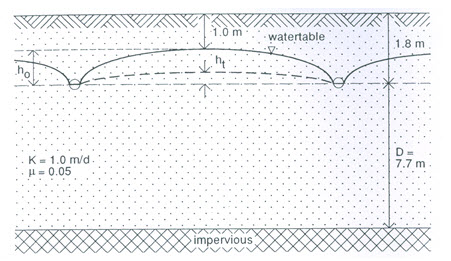
Fig. 7.3. Calculation of drain spacing under unsteady-state conditions. (Source: Ritzeman, 1994)

(1)  Agricultural drainage criteria:

• The maximum permissible height of the water table is 1 m below the soil surface; and

• Irrigation water is applied every 10 days, and the field application losses percolating to the water table are 25 mm for each irrigation.

(2)  Technical design criteria:

• Drains are installed at a depth of 1.8 m; and

• PVC drain pipes with a radius of 0.10 m are used.

(3)  Soil data:

• The depth of the impervious layer is 9.5 m below the soil surface; and

• The average hydraulic conductivity of the soil is 1.0 m/day and the drainable porosity is 0.05.

Solution:

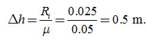
If we assume that the field application losses can be regarded as an instantaneous recharge, R_i = 0.025 m, the rise of the water table computed as:

If we assume that, after irrigation, the water table rose to its maximum permissible height, we know

Thus, we have the following data:

K = 1.0 m/day,  m = 0.05,  D = (9.5 – 1.8) m = 7.7 m,  r₀ = 0.10 m,  h₀ = 0.8 m, h₁₀ = 0.3 m, and t = 10 days

Substituting the above values into the Glover-Dumm drainage equation  

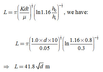
As we know with the help of D, r₀ and L, we can obtain the equivalent depth d from Table 6.1 (Lesson 6). Thereafter, L can be computed by the trial-and-error method:

First Trial: Assume L = 80 m, and with D = 7.7 m, d is found from Table 6.1 (Lesson 6) as:

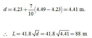
which is more than 80 m (assumed value of L), and hence the spacing is too large.

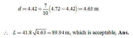
Second Trial: Assume L = 90 m, and with D = 7.7 m, d is found from Table 6.1 as:

7.4  Comparison of Steady-State and Unsteady-State Equations

The question of whether to use the steady-state or the unsteady-state approach to calculate the required drain spacing depends mainly on the availability of data (Ritzema, 1994). Table 7.1 summarizes the input data required for the steady-state and unsteady-state equations.

Table 7.1. Input data for steady-state and unsteady-state drainage equations (after Ritzema, 1994)

Input Data	Steady-State Equations	Unsteady-State Equations
(i)    Soil Data: Profile description Hydraulic conductivity Drainable porosity	Yes Yes No	Yes Yes Yes
(ii)   Agricultural Criteria: q/h ratio h0/ht ratio	Yes No	No Yes
(iii)     Technical Criteria: Drain depth, pipe size, etc.	Yes	Yes

To apply the drainage equations, we have to simplify the soil profile. We have already mentioned that unsteady-state equations can only be applied if a homogeneous soil profile is assumed; for a layered soil profile, steady-state equations have to be used. In both the cases, the hydraulic conductivity which is considered to be constant within each soil layer should be known. On the other hand, for unsteady-state equations, the drainable porosity is also required. As it is even more complicated to measure the drainable porosity than the hydraulic conductivity, the applicability of unsteady-state equation is somewhat limited.

In the unsteady-state approach, the agricultural criterion is based on the rate of water table drawdown (h₀/h_t) instead of a water table discharge criterion (q/h) as in the steady-state approach. The agricultural criteria are often based on relationships that only take the variation in depth of the water table into consideration. Thus, it can be concluded that, on the one hand, steady-state equations are preferred because relatively less soil data are required, but, on the other hand, the agricultural criteria are often based on the variation in the depth of the water table. Fortunately, it is possible to combine the two approaches because the corresponding criteria can be converted into one another (Ritzema, 1994).

Let’s consider the following Hooghoudt Equation which assumes flow below the drain level only:

In the unsteady-state equations, the design criteria are expressed in the reaction factor (a) as:

Combining these two equations by eliminating L yields the following equation

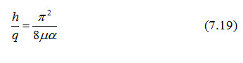
Where, all symbols have the same meaning as defined earlier.

Using Eqn. (7.19), it is possible to establish the unsteady state criteria (i.e., the regard drawdown of the water table in a certain period of time) in experiments on a pilot scale. These unsteady-state criteria can be converted into steady-state criteria, which can be applied on a project scale. In this way, it is not necessary to measure the drainable porosity on a project scale, which is virtually impossible in practice.

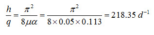
Illustrative Example (Ritzema, 1994): We can also solve Example Problem 1 in an indirect way by converting the unsteady-state drainage criterion h₀/h_t into a steady-state criterion q/h. We know the rate of drawdown of the water table over a period of 10 days. Therefore, we can calculate the reaction factor using Eqn. (7.9) as:

By applying Eqn. (7.19), we can convert this unsteady-state criterion into a steady-state criterion as follows:

Neglecting the flow above the drain level, we can now calculate the drain spacing by using the simplified Hooghoudt Equation:

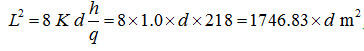
which can be solved by the trial-and-error method.

First Trial: Assume L = 90 m, and we have D = 7.7 m, d = 4.63 m (from Example Problem 1). Thus,

   L² = 1746.83 ´ 4.63 = 8087.84 m²

   L = 89.93 m, which is acceptable.

Note: The reaction factor (a) is a function of the parameters L, K, d, and m (Equation 7.6). Except for the drain spacing (L), these parameters are difficult to establish. The above example shows that an alternative way of obtaining a is by monitoring the drawdown of the water table after a sudden rise (e.g., caused by irrigation or heavy rainfall). In this example, a was calculated only from the water table level at t = 0 and t = 10 days. If more data are available, a can be found by an exponential regression (Ritzema, 1994).

References

De Zeeuw, J.W. and Hellinga, F. (1958). Neerslag en afvoer. Landbouwkundig Tijdschrift. 70, pp. 405-422 (in Dutch with English summary).

Dumm, L.D. (1954). Drain spacing formula. Agricultural Engineering 35, pp. 726-730.

Dumm, L.D. (1960). Validity and use of the transient flow concept in subsurface drainage. Paper presented at ASAE Meeting, Memphis, December, pp. 4-7.

Ritzema, H.P. (1994). Subsurface Flow to Drains. In: H.P.Ritzema (Editor-in-Chief), Drainage Principles and Applications, International Institute for Land Reclamation and Improvement (ILRI), ILRI Publication 16, Wageningen, The Netherlands, pp. 283-304.

Smedema, L.K. and Rycroft, D.W. (1983). Land Drainage: Planning and Design of Agricultural Drainage Systems. Batsford, London, 376 pp.

Suggested Readings

Murty, V.V.N. and Jha, M.K. (2011). Land and Water Management Engineering. Sixth Edition, Kalyani Publishers, Ludhiana, India.

Ritzema (Editor-in-Chief) (1994). Drainage Principles and Applications. International Institute for Land Reclamation and Improvement (ILRI), ILRI Publication 16, Wageningen, The Netherlands.

Schwab, G.O., Fangmeier, D.D., Elliot, W.J. and Frevert, R.K. (2005). Soil and Water Conservation Engineering. Fourth Edition, John Wiley and Sons (Asia) Pte. Ltd., Singapore.

Smedema, L.K. and Rycroft, D.W. (1983). Land Drainage. Batsford Academic and Educational Ltd., London.