Ground Water,Wells and Pumps 3(2+1)

Lesson 20 Evaluation of Groundwater Potential and Quality

      (20.1)

 Where, D_AQ = depth to the aquifer base [L], D_WT = depth to water table in the pre-monsoon season [L], A_Q = areal extent of the aquifer [L²], and S_Y = specific yield of the aquifer [fraction].

Depth to the aquifer base is estimated with the help of borewell (well log) data of multiple sites over the area under study (basin or sub-basin). Depth to water table can be measured by water-level indicator or water-level recorder. Areal extent of the aquifer can be estimated from the groundwater fluctuation data of multiple sites. The best method for determining specific yield is the field pumping test. It should be noted that Eqn. (20.1) can also be used to estimate static groundwater reserve at a site or in a zone.

 20.1.2 Estimation of Dynamic Groundwater Reserve

‘Dynamic groundwater reserve’ refers to the long-term average annual recharge under conditions of maximum groundwater use (GWREC, 1997). Generally up to the end of October, the soil is saturated with moisture and no additional groundwater for irrigation is required. Groundwater irrigation actually starts from the beginning of November and continues until May of the next year. Therefore, the dynamic groundwater reserve (DGWR) can be estimated as follows (GWREC, 1997):

 DGWR = (D_WTE - D_WTO) × A_Q× S_Y                     (20.2)

 Where, D_WTE = depth to water table in the pre-monsoon season of next year [L], D_WTO = depth to water table in the post-monsoon season of the current year [L], A_Q = areal extent of the aquifer [L²], and S_Y = specific yield of the aquifer [fraction].

 Eqn. (20.2) can be used to estimate dynamic groundwater reserve at a site or in a zone. It is worth mentioning that the dynamic groundwater reserve is also called exploitable groundwater reserve or utilizable groundwater reserve, which means that this amount of groundwater can be fully withdrawn to meet water demands in a year without causing any detrimental effect on the available groundwater reserve.

 In general, the pre-monsoon season for a particular year refers to the period from October/November of previous year to the May/June of the particular year, whereas the post-monsoon season for a particular year refers to the period from October/November of that year until May/June of next year. However, for calculating dynamic groundwater reserve using Eqn. (20.2), the depth to water table in the month of May/June is taken as representative for the pre-monsoon season and the depth to water table in the month of October/November is taken as representative for the post-monsoon season. For the purpose of groundwater assessment in India, the monsoon season can be taken as May/June to September/October for all the areas of India except those areas where predominant rainfall occurs during the Northeast monsoon season. An additional period of one month after the cessation of monsoon is taken into account for the baseflow or groundwater recession which occurs immediately after the monsoon season (GWREC, 1997). In the areas (e.g., Tamil Nadu, parts of Kerala)  where predominant rainfall is due to Northeast monsoon, the period of recharge assessment is based on pre-monsoon (October) to post-monsoon (February) water table fluctuations (GWREC, 1997).

 Note that the static or dynamic groundwater reserve in an area/basin should be calculated zone-wise after dividing the area/basin into suitable zones and then computing static groundwater reserve or dynamic groundwater reserve in each zone on a yearly basis. The annual estimates of static/dynamic groundwater reserve, if necessary, could be used to calculate average values of static/dynamic reserve in each zone. A user-friendly computer software package named GWARA has been developed by Prof. Madan Kumar Jha, IIT Kharagpur (developer of this course), which facilitates the assessment of static and groundwater potential at a basin or sub-basin scale as well as the estimation and analysis of groundwater recharge.     

 20.1.3 Assessment of Status of Groundwater Development

Status/Level of Groundwater Development (GWD) is defined as (GWREC, 1997):

 

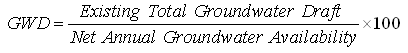             (20.3)

 

The term ‘Net annual groundwater availability’ refers to the available annual recharge after allowing for natural groundwater discharge in the monsoon season in terms of baseflow and/or groundwater outflow. ‘Existing total groundwater draft’ refers to the sum of groundwater withdrawals for different uses (i.e., irrigation, domestic, industry, etc.). Using Eqn. (20.3), a groundwater basin or sub-basin can be categorized based on the level/extent of groundwater extraction/exploitation (development) as shown in Table 20.1 (GWREC, 1997).

 

Table 20.1. Guidelines for assessing the extent of groundwater development

(Source: GWREC, 1997)

Sl. No.	Category	Level of Groundwater Development
1	White Zone/Region	< 65%
2	Grey Zone/Region	65 to 85%
3	Dark Zone/Region	85 to 100%
4	Overexploited Zone/Region	>100%

 

Besides the guidelines provided in Table 20.1 for evaluating the status of groundwater development, it has been recommended that long-term trend of groundwater levels in an area or basin should also be analyzed (GWREC, 1997) for an efficient evaluation of the status/level of groundwater extraction. A graph is prepared showing annual variation of pre-monsoon and post-monsoon groundwater levels for a minimum period of 10 years. The trends of both pre-monsoon and post-monsoon groundwater levels are depicted in the same graph. The trends of these two types of groundwater-level plots are used to interpret the scope of further groundwater development/exploitation with the help of standard guidelines suggested by GWREC (1997). This exercise can be performed for planning future groundwater resources development in a basin/sub-basin concerning additional withdrawal of existing groundwater resources.

20.2 Water Quality and Groundwater Contamination

20.2.1 Water Chemistry vis-à-vis Water Quality

The quality of water that we drink as well as the quality of water in our lakes, streams, rivers, and oceans is a critical parameter in determining the overall quality of our lives. Water quality is determined by the solutes and gases dissolved in the water, as well as the matter suspended in and floating on the water. Water quality is a consequence of the natural physical, chemical and biological state of water as well as of the changes occurred due to human activities. It determines the usefulness of water for a particular purpose. If human activities alter the natural water quality so that it is no longer suitable for a use for which it had been suited earlier, the water is said to be polluted or contaminated. It should be noted that in many regions of the world, water quality has been altered by human activities, but the water is still usable; though ever-growing pollution of both surface water and groundwater is posing a serious threat to our life and ecosystems throughout the world.

 

One basic measure of water quality is the total dissolved solids (TDS), which is the total amount of solids (in milligrams per liter) left when a water sample is evaporated to dryness. Table 20.2 shows the classification of water based on TDS (Fetter, 1994). Water naturally contains a number of different dissolved inorganic constituents. The major cations are calcium, magnesium, sodium, and potassium; the major anions are chloride, sulfate, carbonate, and bicarbonate. Although not in ionic form, silica can also be a major constituent. These major constituents constitute the bulk of the mineral matter contributing to total dissolved solids (TDS). In addition, there may be minor constituents present in water such as iron, manganese, fluoride, nitrate, strontium, and boron. Trace elements such as arsenic, lead, cadmium, and chromium may be present in amounts of only a few micrograms per liter, but they are very important from a water-quality viewpoint because of their harmful effects on human health.

 

Table 20.2 Classification of water based on TDS

(Source: Fetter, 1994)

Sl. No.	Water Class	Value of TDS (mg/L)
1	Fresh	0-1,000
2	Brackish	1,000-10,000
3	Saline	10,000-100,000
4	Brine	>100,000

 

Furthermore, dissolved gases are present in both surface water and groundwater. The major gases of concern are oxygen and carbon dioxide. Nitrogen, which is more or less inert, is also present. Minor gases of concern are hydrogen sulfide and methane. Hydrogen sulfide is toxic and imparts a bad odor, but it is not present in the water that contains dissolved oxygen (DO).

Surface water may be adversely impacted by human activities. If organic matter, such as untreated human or animal waste, is placed into the surface water body, dissolved oxygen (DO) levels diminish as microorganisms grow using organic matter as an energy source and consuming oxygen in the process. The total dissolved solids (TDS) may increase due to the disposal of wastewater, urban runoff, and increased erosion due to land-use changes in a river basin. Generally groundwater has higher dissolved mineral concentrations than surface water because of the extended contact time between groundwater and rocks and soils.

The natural quality of groundwater varies substantially from place to place. It can range from total dissolved solids contents of 100 mg/L or less for some fresh groundwater to more than 100,000 mg/L for some brine found in deep aquifers (Fetter, 1994). Taking this variability into account, the U.S. Environmental Protection Agency (U.S. EPA) has developed a three-part classification system for the groundwater of the United States (U.S. EPA, 1984).

Class I: Special Groundwaters are those that are highly vulnerable to contamination because of the hydrological characteristics of the areas under which they occur and that are also either an irreplaceable source of drinking water or ecologically vital because they provide baseflow for a particularly sensitive ecosystem.

Case II: Current and Potential Sources of Drinking Water and Waters Having Other Beneficial Uses are all other groundwaters except Class III.

Class III: Groundwaters Not Considered Potential Sources of Drinking Water and of Limited Beneficial Use because the salinity is greater than 10,000 mg/L or the groundwater is otherwise contaminated beyond levels that can be removed using methods reasonably employed in public water-supply treatment.

The U.S. EPA uses the above classification scheme in promulgating rules and regulations at the federal level (Fetter, 1994). The highest degree of protection is given to Class I groundwater.

Note that the pollution of surface water frequently results in a situation where the contamination can be seen or smelled. However, the contamination of groundwater most often results in a situation that cannot be detected by human senses. Groundwater contamination can be due to bacteriological or toxic agents or simply due to an increase in common chemical constituent to a concentration whereby the usefulness of the water is impaired.

20.2.2 Sources of Groundwater Contamination

Humans have been exposed to hazardous substances dating back to prehistoric times when they inhaled noxious gases from volcanoes and in cave dwellings. Pollution problems started in the industrial sector with the production of dyes and other organic chemicals developed from the coal tar industry in Germany during the 1800s (Bedient et al., 1999). In the 1900s, a variety of chemicals and chemical wastes increased drastically from the production of steel and iron, lead batteries, petroleum refining and other industrial practices. During that time, radium and chromic wastes also started creating serious quality problems. The World War II era ushered in a massive production of wartime products that required use of chlorinated solvents, polymers, plastics, paints, metal finishing, and wood preservatives (Bedient et al., 1999). Very little was known those days about the environmental impacts of many of these chemical wastes; only after several years, the impacts of various chemical wastes, municipal wastes and other chemicals could be known. Presently, there is a serious concern for the degradation of environment due to deteriorating water and air quality in both developed and developing nations.

 Table 20.3 presents a list of major organic contaminants according to the Environmental Protection Agency (EPA). This is the target list of 126 priority pollutants defined by EPA for their contract laboratory program. The volatile compounds are determined by standard EPA method 624, the semivolatiles by method 625, and pesticides and PCBs by method 608 (Bedient et al., 1999).

Table 20.3. Sources of groundwater contamination

(Source: Bedient et al., 1999)

Category I	Category II	Category III
Sources designed to discharge substances	Sources designed to store, treat, and/or dispose of substances; discharge through unplanned release	Sources designed to retain substances during transport mission
-  Subsurface percolation (e.g., septic tanks and cesspools) -  Injection wells -  Land application	-   Landfills -   Open dumps -   Surface impoundments -   Waste tailings -   Waste piles -   Materials stockpiles -   Above ground storage tanks -   Underground storage tanks -   Radioactive disposal sites	-  Pipelines -  Materials transport and transfer
Category IV	Category V	Category VI
Sources discharging as consequence of other planned activities	Sources providing conduit or inducing discharge through altered flow patterns	Naturally occurring sources whose discharge is created and/or exacerbated by human activities
-  Irrigation practices -  Pesticide applications -  Fertilizer applications -  Animal feeding operations -  De-icing salts applications -  Urban runoff -  Percolation of atmospheric pollutants -  Mining and mine drainage	-    Production wells -    Other wells (non-waste) -    Construction excavation	-     Groundwater-surface water interactions -     Natural leaching -     Salt-water intrusion/brackish water upconing due to pumping

 

Fig. 20.1 shows the various mechanisms of groundwater contamination associated with some of the major sources. These sources are: chemical and fuel underground storage tanks, septic tanks, municipal landfills, and surface impoundments. A wide variety of organic and inorganic chemicals coming from both natural and man-made sources have been identified as potential contaminants in groundwater. They include inorganic compounds such as nitrates, brine, and various trace metals; synthetic organic chemicals such as fuels, chlorinated solvents, and pesticides; radioactive contaminants associated with defense sites; and pathogens.

 

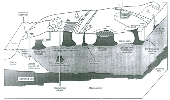
Fig. 20.1. Mechanisms of groundwater contamination.

(Source: Bedient et al., 1999) 

The detailed discussion on the sources of groundwater contamination, the properties/characteristics of various organic and inorganic compounds identified as major threats to groundwater, and their impacts on groundwater can be found in Bedient et al. (1999), Todd (1980) and Fetter (1994).

20.2.3 Water Quality Standards

Chemical analyses are widely used to determine the suitability of water for different purposes such as drinking, irrigation, industrial and ecosystems. For this, we require sets of standards based on which the quality of given water can be evaluated. These standards change from time to time and vary from country to country.

Water-quality standards are the regulations that set specific limitations on the quality of water which may be applied to a specific beneficial use. Water-quality criteria are the values of dissolved substances in water and their toxicological and ecological meaning. These data are often used to set water-quality standards. Two sets of water-quality standards gained international status in early seventies (Roscoe Moss Company, 1990): (i) World Health Organization (WHO) International Standards, and (ii) WHO European Standards. The WHO International Standards were intended as minimal standards and were considered to be achievable by all countries of the world. The WHO European Standards were more rigorous and reflected the water treatment technologies available to developed nations. Recognizing the many social, economic and cultural constraints of implementing uniform international standards, WHO developed a comprehensive set of guidelines for drinking water quality in 1984. These supersede the formal European and International Standards and instead provide a basis on which individual countries can develop standards and regulations of their own. Nevertheless, the WHO International Standards (WHO, 2006) are updated from time to time and are often used in many countries, especially in developing countries.

Besides the WHO standards, the rigorous U.S. Environmental Protection Agency Standards have also achieved almost an international recognition. Apart from the drinking-water standards, there exist separate water-quality standards for irrigation (Ayers and Westcot, 1985) as well as different industrial uses (Roscoe Moss Company, 1990), together with the water-quality standards for livestock consumption and that for maintaining the health of aquatic ecosystems.

Drinking water standards are especially important for evaluating groundwater quality because many consumers utilize untreated groundwater that is directly pumped from a well. Public water-supply systems that rely on groundwater are required to perform a complete analysis of the water for the drinking-water standards prior to the time a well is put into service and periodically thereafter. Private wells are often tested for bacteria and nitrate only when they are first drilled and then never tested again (Fetter, 1994). It is very important to maintain high quality in groundwater in order to protect private well owners. The situation of water-quality monitoring and its protection is much worse in many developing countries, including India. On the other hand, the important issues involved in using water for irrigation are requirements to match the salinity of irrigation water to the salt tolerance of selected crops, to avoid salt buildup in the soil, and to avoid a breakdown of the soil structure and a reduction in permeability by using water having high sodium concentration.

 20.3 Collection of Water Samples

This section focuses on the methods of collecting representative water samples for chemical analyses in a specialized analytical laboratory. The program to sample both groundwater and surface water must be carefully planned considering the purpose of water sampling, number of sampling points, types of chemical constituents to be analyzed, frequency of sampling and the quality assurance/quality control (QA/QC) issues. In contamination studies or research investigations, wells are usually installed to provide samples from specified locations and to assure the quality of the sample. In this case, an investigator must make decisions concerning the location of the wells, their design, and the method of installation (Schwartz and Zhang, 2003). Making appropriate decisions in this respect can minimize potential errors in water sampling.

 20.3.1 Methods of Groundwater Sampling

Sampling is a critical step in obtaining valid water-quality data. A sample must be representative of the water residing in an aquifer (or produced from a well), and its integrity must be maintained until the laboratory tests are completed. Note that water standing in a well casing is probably not representative of the overall groundwater quality. This can be due to the presence of drilling contaminants, biological growths, and corrosion by-products or changes in environmental conditions such as redox potential. For these reasons it is necessary to pump or bail a well before collecting water samples. The recommended time of pumping depends on several factors, including the hydrogeology of the aquifer, the constituents or parameters to be tested, and the characteristics of the well. For small monitoring wells that are not easily bailed, a common practice is to pump or bail the well until a minimum of 4 to 10 bore volumes have been removed (Roscoe Moss Company, 1990). If possible, it is desirable to pump a production well for one to two hours before collecting water samples.

Newly completed wells sometimes require extended periods of pumping before a truly representative sample can be obtained. Samples collected during the first few hours of operation may be of a different quality than the samples collected after several days. This phenomenon has been observed in wells that penetrate more than one aquifer (Roscoe Moss Company, 1990). Sampling protocols or Standard operating procedures (SOPs) have been developed by the U.S. EPA and other government agencies. They specify the type of sample that is needed (grab or composite), the type of container that is to be used for the sample, the method by which the sample container is cleaned and prepared, whether or not the sample is filtered, the type of preservative that is to be added to the sample in the field, and the maximum time period for holding the sample prior to analysis in the laboratory. Based on these sampling protocols, Fetter (1994) and Schwartz and Zhang (2003) present useful guidance on groundwater sampling protocols, together with the design and installation of monitoring wells, sampling techniques, and the quality assurance/quality control (QA/QC) program.

It is a good field practice to clean thoroughly the sampling device prior to use. The method of cleaning should be such that no residue remains. The sampling devices and bottles should be rinsed with a sample of the water being sampled, if they are not thoroughly dry. This avoids the mixing of rinse water with the final water sample. Many of the chemical, physical and biological parameters in groundwater are unstable. Therefore, proper care should be taken in maintaining water sample integrity. Various sources of error involved in water sampling are described in the subsequent sub-section.

20.3.2 Sources of Error

Collecting water samples involves several steps, and problems can arise in each step. The groundwater sampling process begins by taking water from wells using a bailer or a pump. After bringing a groundwater sample to the surface, a few parameters like pH and specific conductance are measured immediately with portable equipment. Water is also stored in various containers, some of which could be special containers or contain preservatives to prevent deterioration. Many types of analyses require that the samples be chilled on ice and then transported to an appropriate laboratory for analyses. Although these steps appear to be simple, there may be a number of pitfalls and problems which

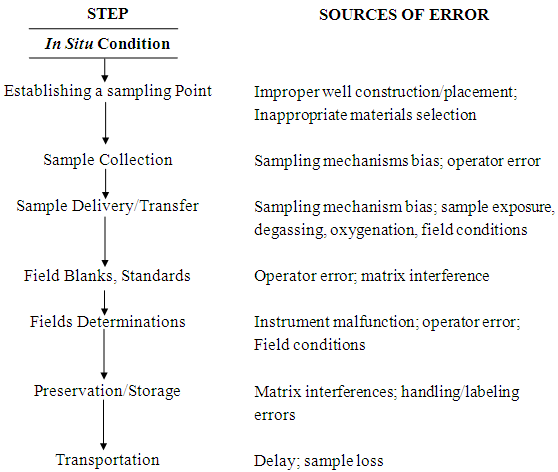
Fig. 20.2. Steps in groundwater sampling and sources of error.

(Source: Schwartz and Zhang, 2003)

can invalidate the sample results.  Fig. 20.2 summarizes the sources of errors in sampling groundwater. They include improper procedures for installing the well, reactions between the groundwater and the well casing or sampler, and poor sample-handling protocols on the surface. Following the standard procedures of water sampling and their strict adherence during sampling can minimize these errors. Unfortunately, some problems can happen to a water sample even after reaching the analytical laboratory (Schwartz and Zhang, 2003). These problems encompass the errors due to deterioration of samples and laboratory standards, and the poor analytical methods. The laboratory problems also require that QC checks be designed to detect errors that originate in the laboratory.

 20.4 Analysis of Water Quality

Describing the concentration of major and minor cations and anions, and the pattern of water quality variability is part of many groundwater investigations. A variety of graphical and statistical techniques are presently available for analyzing water quality data. Machiwal and Jha (2010) present a review of various tools and techniques for the analysis of water quality data as well as some case studies demonstrating the application of some of these techniques. Each technique has certain advantages and disadvantages in representing features of the data. Therefore, researchers/hydrogeologists should select appropriate tools and techniques for the effective analysis of water-quality data.

In short, the methods of water quality analysis can be divided into three major groups: (a) First group comprises a set of graphical methods for describing abundance or relative abundance, (b) Second group comprises methods that present patterns of variability in addition to abundance, and (c) Third group comprises derived maps that involve various types of calculations with the basic data. A brief discussion about these methods is provided below.

 20.4.1 Graphical Methods

Several different graphical approaches can depict the abundance or relative abundance of ions in individual water samples. The most common approaches are: (i) Collins bar diagram, (ii) Stiff pattern diagram, (iii) pie diagram, and (iv) Piper diagram. In these plots, concentrations need to be expressed as meq/L or %meq/L. The Collins and Stiff diagrams require absolute concentrations (meq/L), whereas the pie and Piper diagrams require relative concentrations (%meq/L). Figs. 20.3(a, b, c, d) illustrate the sample data plotted in four different ways. The Collins, Stiff, and pie diagrams are relatively simple to construct. They require only that concentrations be plotted as a bar segment, a point on a line, or a percentage of the pie. The appropriate fields are shaded and possibly labeled in the case of the Collins and Piper diagrams (Fig. 20.3). The Stiff diagram can be plotted with or without the labeled axes.

 

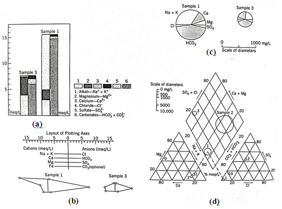
Fig. 20.3. Four different ways of plotting major ion data: (a) Collins diagram; (b) Stiff diagram; (c) Pie diagram; (d) Piper diagram.

(Source: Schwartz and Zhang, 2003)

 

Plotting data for a Piper diagram is complicated because there are three separate diagrams (Fig. 20.3d). The relative abundance of cations with the %meq/L of

Na⁺ + K⁺, Ca²⁺, and Mg²⁺ assumed to equal 100% is first plotted on the cation triangle. Similarly, the anion triangle displays the relative abundance of Cl^-, and. Straight lines projected from the two triangles into the quadrilateral field define a point on the third field (Fig. 20.3d). To provide some indication of the absolute quantity of dissolved mass in the sample, the size of the data point is sometimes related to the salinity (TDS).

One advantage of all four techniques is that they present the major ion data for a sample on one figure. However, with the exception of the Piper diagram, these approaches are useful only in displaying the results for a few analyses. Presenting a large number of these diagrams together is confusing and is not much more helpful than showing concentration values in a tabular form (Schwartz and Zhang, 2003).

20.4.2 Other Methods

Graphical/illustrative type diagrams or statistics can define the pattern of spatial change among different geologic units, along a line of section, or along a pathline (Schwartz and Zhang, 2003). The simplest way for representing spatial variation of water quality over a particular geological layer is to take the single sample diagrams (e.g., pie or Stiff) and place them on a map. Such maps can show how the pattern of ion abundances changes within a given geological unit. Showing all the chemical constituents on a single map is often helpful.

When the water-quality data (measured or computed) vary systematically in space, it is often best to plot contour concentrations (or other data) on maps or cross sections (Fig. 20.4). This type of presentation clearly depicts the variation of individual parameters. However, this type of presentation involves a large number of figures to completely describe the chemistry of an area. Furthermore, GIS techniques can be used to effectively perform spatio-temporal analysis of water-quality data.

 

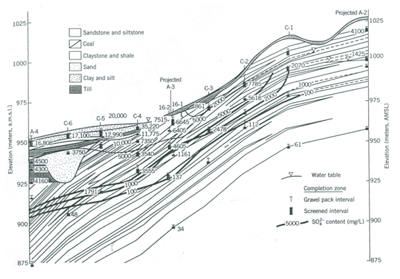
Fig. 20.4. Contours of ion concentration plotted on a cross section.

(Source: Schwartz and Zhang, 2003)

If the water-quality data are ‘noisy’, a Piper diagram is preferable to concentration maps. By classifying samples on the Piper diagram, one can identify geologic units with chemically similar water and define the evolution in water chemistry along a flow system (Schwartz and Zhang, 2003). Also, noisy water-quality data can be smoothed before plotting on a map or geological cross-section. The facies mapping approach provides one way of smoothing chemical data (Schwartz and Zhang, 2003).

 Apart from the above methods of water-quality analysis, the statistical techniques such as time series analysis, t-test, regression/correlation analysis, multivariate analysis, etc. are also very useful and are being used by several researchers.

 References

• Ayers, R.S. and Westcot, D.W. (1985). Water Quality for Agriculture. FAO Irrigation and Drainage Paper 29 Rev. 1, Food and Agriculture Organization (FAO), Rome, Italy. 

• Bedient, P.B., Rifai, H.S. and Newell, C.J. (1999). Ground Water Contamination: Transport and Remediation. 2^nd Edition, Prentice Hall, N.J.

• Fetter, C.W. (1994). Applied Hydrogeology. Third Edition, Prentice Hall, N.J.

• GWREC (1997). Report of the Ground Water Resource Estimation Committee (GWREC). Central Ground Water Board, Ministry of Water Resources, Government of India, New Delhi.

• Machiwal, D. and Jha, M.K. (2010). Tools and techniques for water quality interpretation. In: G. Krantzberg, A. Tanik, J.S.A. do Carmo, A. Indarto and A. Ekdal (Editors-in-Chief), Advances in Water Quality Control, Chapter 9, Scientific Research Publishing, Inc., California, USA, pp. 211-251.

• Roscoe Moss Company (1990). Handbook of Ground Water Development. John Wiley & Sons, New York.

• Schwartz, F.W. and Zhang, H. (2003). Fundamentals of Ground Water. John Wiley & Sons, New York.

• Todd, D.K. (1980). Groundwater Hydrology. John Wiley & Sons, New York.

• U.S. EPA (1984). A Ground Water Protection Strategy for the Environmental Protection Agency. United States Environmental Protection Agency (U.S. EPA), Washington, D.C.

• WHO (2006). Guidelines for Drinking-Water Quality: First Addendum to Third Edition. Volume 1, Recommendations, World Health Organization (WHO), Geneva, Switzerland.

 

Suggested Readings

• Todd, D.K. (1980). Groundwater Hydrology. John Wiley & Sons, New York.

• Bedient, P.B., Rifai, H.S. and Newell, C.J. (1999). Ground Water Contamination: Transport and Remediation. 2^nd Edition, Prentice Hall, N.J.

• Schwartz, F.W. and Zhang, H. (2003). Fundamentals of Ground Water. John Wiley & Sons, New York.

• Fetter, C.W. (1994). Applied Hydrogeology. Third Edition, Prentice Hall, N.J.

• Sarma, P.B.S. (2009). Groundwater Development and Management. Allied Publishers Pvt. Ltd., New Delhi.