Irrigation Engineering 4(3+1)

LESSON 33 Border Irrigation System

33.1 General Adaptability

Border irrigation is suited to all crops that are not damaged by inundation for short periods. It can be used on nearly all irrigable soils but is best suited to soils whose intake rates are neither extremely low nor extremely high.

 

33.2 Design Considerations

33.2.1 Layout

The border strips are so located that a supply channel or pipeline delivers water to the upper end of the border. It is also suggested that the border strips are constructed parallel to the filed boundary to facilitate the intercultural operations. For long fields with soils having high infiltration capacity more than one border strip should be constructed along the entire length of the field.  The main factors to be considered during the design of layout are given below:

 

33.2.2 Water Source Location

It is desirable to choose a water source in the central position of the filed to minimize the construction of channel and pipes also keeping in mind the fact that the water source should be in a position to facilitate the gravity flow to the field channels.

 

33.2.3 Border Strip Width

-         Border strip widths suitable for any particular field depend on (1) available stream size (2) amount of cross slope that must be removed, (3) kind of equipment used, and (4) accuracy of land levelling as related to the normal depth of flow expected.

-         The width of a border usually varies from 3 to 15 meters, depending on the size of irrigation stream available and the degree of land levelling practicable.

 

33.2.4 Border Strip Length

Longer border strip are desirable to reduce the labour and other operating costs, however the aspect of uniformity and application efficiency of the border strip should be kept in mind while determining the length of the border. Long border strips are easier to farm than short strips because fewer turns by farm equipment are required. Soil type is the most important aspect which determines the length of the border. Typical border lengths for different soils are given in Table 33.1

 

Table 33.1. Recommended border length for different type of soil for moderate slopes and small to moderate size irrigation streams

Type of soils	Border length, (m)
Sand	60 to 90
Loamy sand	75 to 150
Sandy loam	90 to 250
Clay loam	90 to 300
Clay	180 to 350

 

33.2.5 Land Smoothening

Land smoothening increases the efficiency by eliminating any furrows in which the flow might accumulate. Borders with zero cross slopes are preferred for higher irrigation efficiencies however in undulating terrain cross slopes might be present. While levelling the land the topography must be studied carefully to economize the operation by levelling the smaller slopes.

 

33.2.6 Stream Size

The design stream size should be large enough to spread adequate amounts of water across the length and breadth of the border; however it should be erosive in nature. The design stream size should also result in rates of advance and recession which are essentially equal.

-         The size of irrigation stream needed depends on the infiltration rate of the soil and the width of the border strip.

-         The depth of water applied to the soil can be regulated by the size of the irrigation stream.

 

Table 33.2. Some typical values of stream sizes to suit varying soil characteristics and border slopes

Soil Type	Border Slope (%)	Flow per metre width of border strip, litre per second
Sandy soil, infiltration rate 2.5 cm per hour	0.20-0.40 0.40-0.65	10-15 7-10
Loamy sand, infiltration rate 1.8 to 2.5 cm per hour	0.20-0.40 0.40-0.60	7-10 5-8
Sandy loam, infiltration rate 1.2 to 1.8 cm per hour	0.20-0.40 0.40-0.60	5-7 4-6
Clay loam, infiltration rate 0.60 to 0.80 cm per hour	0.15-0.30 0.30-0.40	3-4 2-3
Clay, infiltration rate 0.20 to 0.60 cm per hour	0.10-0.20	2-4

 

33.2.7 Irrigation Time

Irrigation time is the infiltration opportunity time. It is calculated from the empirical equations to calculate depth of infiltration noting that the cumulative infiltration should be able to meet the irrigation requirements.

 

33.2.8 Inflow Time

The inflow time is selected keeping in mind that the desired depth of irrigation be applied in the far end of the border. The inflow time is calculated assuming that the advance and the recession curves are parallel.

 

33.2.9 Border Ridge Height

-         On non-cohesive soils, border ridges with a settled height of more than20 cm are difficult to construct and maintain without making them excessively wide.

-         In addition, where salinity is a problem, salt can accumulate in the ridge crest. The higher the ridge, the more pronounced the salt accumulation is likely to be.

 

33.3 Design of Border Irrigation System

Assumptions

• Surface water profiles at time of cutoff (the time at which water inflow is shutoff to  the field,) as well as  (at the end of depletion and also at the beginning of recession,) are straight lines with end points corresponding to uniform flow conditions (Fig.33.1).

• Depth  at the downstream end remains constant during the depletion phase and runoff () occurs at a constant rate.

• During both depletion and recession phases, the sum of infiltration (I) and runoff () remains equal to the pre cutoff unit inflow rate

 

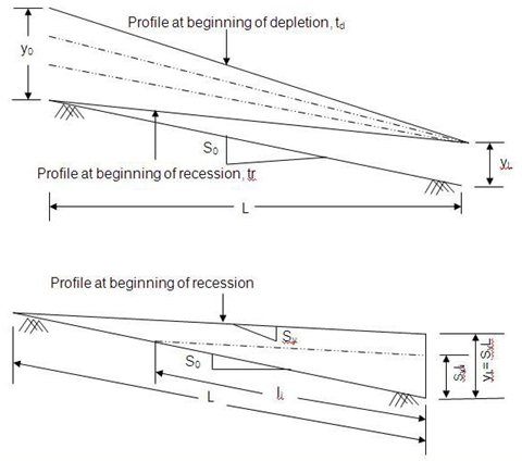
Fig.33.1. Water surface profiles at the beginning of depletion and recession phases.

With these assumption, the time required from the cutoff time to the end of depletion phase, is equal to the time required to remove a triangular volume of length L and height at a constant rate as both infiltration and runoff. It can be expressed as:

                          (33.1)

At the beginning of recession, it is assumed that the depth changes with distance at uniform rate over the entire length of border, which can be expressed as:

                               (33.2)

Where  is function of at time t_d and can be evaluated as follows:

           (33.3)

 

For border, A = y and WP = 1 and therefore R = y or   and I is the average infiltration rate (m/sec) over the length, L.

S_y becomes

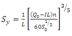     (33.4)

I can be expressed as a mean of infiltration rate at the upstream end (I()) and at the downstream end I(t_d - t_L):

        (33.5)

Walker and Skogerboe (1987) provided an equation for estimating the recession time as follows

        (33.6) 

A step wise design procedure for free drained borders:

1. Collect information related to field characteristics, soil, crop, and water supply.

 

Table 33.3. Data required for the design of basin irrigation systems

Sl. no	Design variables	symbols
1	Kostiakov-Lewis infiltration model parameters	a ,k ,fo
2	Field length	L
3	Field width	Wf
4	field slope	S0
5	Mannings roughness coefficient	n
6	Border shape coefficients	ρ1,p2
7	Required depth of irrigation	Zreq
8	Soil erosive velocity	Vmax
9	Water supply rate	Q
10	Duration of water supply	T

 

2. Determine the maximum (Q_max) and minimum (Q_min)  values of unit inflow rate Q₀  (m³/min/m) using below equation (to limit the flow within the non-erosive velocity with sufficient depth to spread laterally):

 

  (33.7)

                                     (33.8)

 

3. Select unit flow rate ) between  and  in such a way that it results in a set width that contains an even number of borders of satisfactory width and integer number of sets using below equation:

      (33.9)

      (33.10)

4. Compute the inflow depth at the inlet (m) using below equation:

               (33.11)

5. Compute  (min) to satisfy the irrigation requirement from the following equation

  (33.12)

Where Z_reqis the required depth of infiltration.

 6. Compute the time of advance to the end of border (min) (using procedure described in Lecture 31).

7. Compute the time of recession (minutes since the beginning of irrigation) assuming that the design will meet irrigation requirement at the end of the border
 

8. Compute the depletion time  (min) by using Newton Raphson method as follows:

a)    Assume initial guess of t_d as T₁ = t_r

b)   Compute the average infiltration rate along the border by averaging the rates as both ends at time T₁

       (33.13)

c)    Compute the relative water surface slope,

                     (33.14)

d)   Compute a revised estimate of the depletion time,

      (33.15)       

e)   Compare the initial guess, with the new computed value. If both values are equal then  is found and continue with step 9. Otherwise, set and repeat steps b through e.

 

9. Compare the depletion time with the required intake opportunity time. As recession is an important process in border irrigation, it is possible for the applied depth at the end of the field to be greater than at the inlet. If t_d > r_req , the irrigation at the field inlet is adequate and the application efficiency, E_acan be calculated by using the following estimate of time of cutoff

                 (33.16)

        (33.17)

 

10. If  t_d <  r_req the irrigation is not complete and the cutoff time must be increased so the intake at the inlet is equal to the required depth. The computation proceeds as follows

 

              (33.18)

 

 

Example 33.1:

Design a border irrigation system for the following conditions:

Field length, L = 200 m

Field width, W = 100 m,

 

The typical slopes are 0.8% in the 100 m dimension and 0.1% in the other

the Manning roughness coefficient for first irrigations will be taken as 0.04 and for the later irrigations as 0.10

 

Soil texture = silt

Design irrigation requirement = 8 cm

Shape parameters ρ= 1 and ρ₂ = 1.67

Soils appear to be relatively non-erosive and have been tested to yield the following infiltration function:

First irrigation:

Second irrigation:

Infiltration function parameters: k = 0.0053, a = 0.327 and = 0.000052

Available supply rate, Q= 1.8 m³/min

Supply duration =36 hrs.

 

Solution:

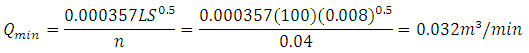
1. Calculate the maximum inflow per unit width for the first irrigation along the 200 m length where erosion is most likely:

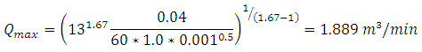
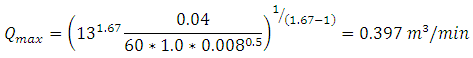
And similarly for irrigations along the 100 m (SO = 0.008) direction

The minimum flow using later field roughness where spreading may be a problem is for the 200 m length

 

Or in the 100 m direction:

 

 

2. Compute  (min) to satisfy the irrigation requirement ,for first irrigation  and for second irrigation

 3. Select  within the range of  and in case of later irrigation

• The flow is adjusted and possible combinations are listed below

 

Number of borders, (Nb)	Border width,(Wb) m	Unit inflow rate (Q0) m³/min/m
1	100	0.018
2	50	0.036
3	33	0.545

 

Q0 = 0.036m³/min/m is selected

4. For an inflow of 0.036 m³/min/m, the advance time along the 200 m length under later conditions is about 301.8 min

5. Compute the inflow depth at inlet (m) using the Mannings equation as follows:

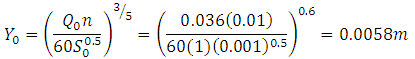
And  value should be less than the ridge height

 6. Compute the time of recession (in minutes since the beginning of irrigation) assuming that the design will meet the irrigation requirement at the end of the border

7. Compute the depletion time  in min using the Newton Raphson method as follows:

a)     Assume an initial estimate of t_d as t_d = t_r = 980.8 min

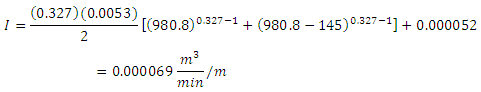
b)    Compute the average infiltration

 

 c)     Compute

 

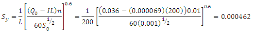
d)    Compute new value of  as  using below equation as follows:

 

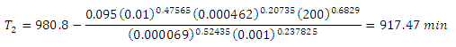
e)     The initial guess () is not close to the new computed value () and repeat step b through e.

8. Correct value of = 802.7 min

9. Compute new  by substituting  in place of in following equation

 

10. Compute application efficiency

 

11. Check the water availability constraint and repeat steps 4 to 10 for other unit inflow rates. Choose the design which gives maximum Ea value.

 

This series of computations is repeated for the full range of discharges, field lengths and infiltration conditions. The following table gives a detailed summary of selected options for the first and subsequent irrigation conditions running in both the 200 m and 100 m directions.

 

First irrigation, L= 200m

Sets	Border width,m	Unit flow,m³/min	Advance time,hr	Cutofftime,hr	Recession time,hr	Field on time,hr	Application efficiency,%
2	50	0.036	6.36	11.34	12.83	22.67	65.3
3	33	0.545	3.11	8.10	9.59	24.29	60.4
4	25	0.072	2.14	7.12	8.61	28.49	52
5	20	0.09	1.64	6.63	8.12	33.16	44.7

 

Later irrigation, L= 200m

Sets	Border width,m	Unit flow,m³/min	Advance time,hr	Cutofftime,hr	Recession time,hr	Field on time,hr	Application efficiency,%
1	100	0.018	15.55	23.66	26.86	23.66	62.6
2	50	0.036	5.03	13.12	16.34	26.24	56.5
3	33	0.0545	3.15	11.25	14.47	33.76	43.4

 

First irrigation, L= 100m

Sets	Border width,m	Unit flow,m³/min	Advance time,hr	Cutofftime,hr	Recession time,hr	Field on time,hr	Application efficiency,%
2	100	0.018	5.27	11.21	11.74	22.42	66.1
3	67	0.0269	2.35	8.30	8.83	24.89	59.8
4	50	0.036	1.44	7.39	7.92	29.55	50.1
5	40	0.045	1.03	6.98	7.51	34.91	40.4

 

 

Later irrigation, L= 100m

Sets	Border width,m	Unit flow,m³/min	Advance time,hr	Cutofftime,hr	Recession time,hr	Field on time,hr	Application efficiency,%
1	200	0.009	12.89	23.07	24.20	23.07	64.2
2	100	0.018	3.45	13.61	14.76	27.23	54.5

 

 

Reference

Michael A.M.(2009), Irrigation Theory and Practice, Vikas publishing House Pvt.Ltd., Delhi.

Walker W. R. and Skogerboe G. V.(1987). Surface Irrigation Theory and Practice. Utah State University, New Jersey 07632.

 

Internet Reference

ftp://ftp.wcc.nrcs.usda.gov/wntsc/waterMgt/irrigation/NEH15/ch5.pdf

http://www.fao.org/docrep/T0231E/t0231e07.htm#5.6 basin irrigation design

 

Suggested Reading

ftp://ftp.wcc.nrcs.usda.gov/wntsc/waterMgt/irrigation/NEH15/ch5.pdf

http://www.fao.org/docrep/T0231E/t0231e07.htm#5.6 basin irrigation design

Michael A.M.(2009), Irrigation Theory and Practice,Vikas Publishing House Pvt.Ltd., Delhi.