Site pages
Current course
Participants
General
Module 1: Introduction and Concepts of Remote Sensing
Module 2: Sensors, Platforms and Tracking System
Module 3: Fundamentals of Aerial Photography
Module 4: Digital Image Processing
Module 5: Microwave and Radar System
Module 6: Geographic Information Systems (GIS)
Module 7: Data Models and Structures
Module 8: Map Projections and Datum
Module 9: Operations on Spatial Data
Module 10: Fundamentals of Global Positioning System
Module 11: Applications of Remote Sensing for Eart...
Lesson 22 Coordinate and Datum System
22.1 Introduction
The oldest global coordinate system is the Latitude/ Longitude system (also referred to as Geographic coordinates). It is the primary system used for determining positions in surveying and navigation. A grid of east-west latitude lines (parallels) and north-south longitude lines (meridians) represent angles relative to standard reference planes. Latitude is measured from 0 to 90 degrees north and south of the equator. Longitude values range from 0 to 180 degrees east or west of the Prime Meridian, which by international convention passes through the Royal Observatory at Greenwich, England Because the Latitude/Longitude system references locations to a spheroid rather than to a plane, it is not associated with a map projection.
Use of latitude/longitude coordinates can complicate data display and spatial analysis. One degree of latitude represents the same horizontal distance anywhere on the Earth’s surface. However, because lines of longitude are farthest apart at the equator and converge to single points at the poles, the horizontal distance equivalent to one degree of longitude varies with latitude. If you have data of regional or smaller extent with Geographic coordinates, you will achieve better results by warping or resampling the data to a planar coordinate system. A large-scale map represents a small portion of the Earth’s surface as a plane using a rectilinear grid coordinate system to designate location coordinates.
A planar Cartesian coordinate system has an origin set by the intersection of two perpendicular coordinate axes and tied to a known location. The coordinate axes are normally oriented so that the x-axis is east-west and the y-axis is north-south. Grid coordinates are customarily referred to as easting (distance from the north-south axis) and northing (distance from the east-west axis). The definition of a Cartesian coordinate system also includes the units used to measure distances relative to these axes (such as meters or feet). For very small areas (such as a building construction site) the curvature of Earth’s surface is so slight that ground locations can be referenced directly to an arbitrary planar Cartesian coordinate system without introducing significant positional errors. For areas larger than a few square kilometers, however, the difference between a planar and curving surface becomes important when relating ground and map locations. A map projection must then be selected to relate surface and map coordinates to reduce undesirable distortions in the map. Cartesian coordinate system is related to the Earth via a map projection is termed a projected coordinate system. A number of projected coordinate systems have been set up to represent large areas (states, countries, or larger areas) by subdividing the coverage area into geographic zones, each of which has its own origin. To minimize variations in scale associated with the map projection, one of the coordinate axes (sometimes both) typically bisects the zone. In that case, in order to force all locations within the zone to have positive coordinate values, a large number is added to one or both coordinates of the origin, termed false easting and false northing. This procedure moves the (0, 0) position of the coordinate system outside the zone to create a false origin, as illustrated in Fig. 22.1. (http://www.microimages.com/documentation/Tutorials/project.pdf)
Many different generic types of coordinate systems can be defined and the calculations necessary to move between them may sometimes be rather complex. In order of increasing complexity they can be thought of as follows. Spherical coordinates are formed using the simplest approximation of a spherical Earth, where latitude is the angle north or south of the equatorial plane, longitude is the angle east or west of the prime meridian (Greenwich) and height is measured above or below the surface of the sphere.
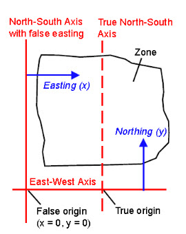
Fig. 22.1. Planar coordinate system with false easting.
(Source: Smith, 2011)
If high accuracy is not important, then this simple model may be sufficient for your purposes. Spheroidal coordinates are formed using a better approximation based on an ellipsoid or spheroid, with coordinates of true latitude, longitude and height; this gives us the system of geodetic coordinates. Cartesian coordinates involve values of x, y and z, and are defined with their origin at the centre of a spheroid. The x and y axes lie in the equatorial plane, with x aligned with the Greenwich meridian, and z aligned with the polar axis. Projection coordinates are then defined using a simple set of x and y axes, where the curved surface of the Earth is transformed onto a plane, the process of which causes distortions. Polar coordinates, generically, are those which are defined by distance and angle, with distance usually denoted r and angle u. Planar coordinates refer to the representation of positions, as identified from polar coordinate positions, on a plane within which a set of orthogonal x, y axes is defined. The conversion between these polar and planar coordinates, for any particular datum, is relatively straightforward and the relationship between them is illustrated in Fig. 22.2. The following expression can be used to derive the distance (d) between two points a and b on an assumed spherical Earth:
![]()
where R is the radius of the Earth, A and B denote the positions of points a and b on the sphere, λ is the longitude and ɸ the latitude. Generically, the x, y (planar) positions of the two points can be derived from the polar coordinates as:
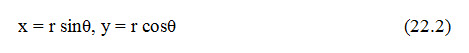
where u is measured clockwise from north. The Pythagorean distance between two points (a and b) can then be found by the following, where the two points are located at (xa, ya and xb, yb):
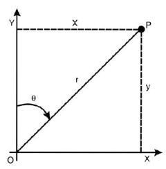
Fig. 22.2. The relationship between polar and planer co-ordinates in a single datum. (Source: Jian and Philippa, 2009)
22.1 Geographic Coordinate System
A geographic coordinate system is a reference system that uses a three-dimensional spherical surface to determine locations on the earth. Any location on earth can be referenced by a point with longitude and latitude coordinates. The values for the points can have the following units of measurement:
-
Linear units when the geographic coordinate system has a spatial reference system identifier (SRID) that DB2(R) Geodetic Extender recognizes.
-
Any of the following units when the geographic coordinate system has an SRID that DB2 Geodetic Extender does not recognize.
-
Decimal degrees
-
Decimal minutes
-
Decimal seconds
-
Gradians
-
Radians
-
For the range of values for these units, refer to Supported coordinate systems. For example, Fig. 22.3 shows a geographic coordinate system where a location is represented by the coordinates longitude 80 degree East and latitude 55 degree North.
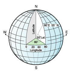
Fig. 22.3. A geographic coordinate system.
(Source:http://publib.boulder.ibm.com/infocenter/db2luw/v9/index.jsp?topic=%2Fcom.ibm.db2.udb.spatial.doc%2Fcsb3022a.html; 3 December 2012)
The lines that run east and west each have a constant latitude value and are called parallels. They are equidistant and parallel to one another, and form concentric circles around the earth. The equator is the largest circle and divides the earth in half. It is equal in distance from each of the poles, and the value of this latitude line is zero. Locations north of the equator have positive latitudes that range from 0 to +90 degrees, while locations south of the equator have negative latitudes that range from 0 to -90 degrees. Fig. 22.4 illustrates latitude lines. The lines that run north and south each have a constant longitude value and are called meridians. They form circles of the same size around the earth, and intersect at the poles. The prime meridian is the line of longitude that defines the origin (zero degrees) for longitude coordinates. One of the most commonly used prime meridian locations is the line that passes through Greenwich, England.

Fig. 22.4. Latitude lines.
(Source:http://publib.boulder.ibm.com/infocenter/db2luw/v9/index.jsp?topic=%2Fcom.ibm.db2.udb.spatial.doc%2Fcsb3022a.html; 3 December 2012)
However, other longitude lines, such as those that pass through Bern, Bogota, and Paris, have also been used as the prime meridian. Locations east of the prime meridian up to its antipodal meridian (the continuation of the prime meridian on the other side of the globe) have positive longitudes ranging from 0 to +180 degrees. Locations west of the prime meridian have negative longitudes ranging from 0 to -180 degrees. Fig. 22.5 illustrates longitude lines.
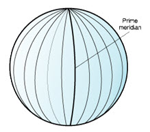
Fig. 22.5. Longitude lines.
(Source:http://publib.boulder.ibm.com/infocenter/db2luw/v9/index.jsp?topic=%2Fcom.ibm.db2.udb.spatial.doc%2Fcsb3022a.html; 3 December 2012)
The latitude and longitude lines can cover the globe to form a grid, called a graticule. The point of origin of the graticule is (0, 0), where the equator and the prime meridian intersect. The equator is the only place on the graticule where the linear distance corresponding to one degree latitude is approximately equal the distance corresponding to one degree longitude. Because the longitude lines converge at the poles, the distance between two meridians is different at every parallel. Therefore, as you move closer to the poles, the distance corresponding to one degree latitude will be much greater than that corresponding to one degree longitude.
It is also difficult to determine the lengths of the latitude lines using the graticule. The latitude lines are concentric circles that become smaller near the poles. They form a single point at the poles where the meridians begin. At the equator, one degree of longitude is approximately 111.321 kilometers, while at 60 degrees of latitude, one degree of longitude is only 55.802 km (this approximation is based on the Clarke 1866 spheroid). Therefore, because there is no uniform length of degrees of latitude and longitude, the distance between points cannot be measured accurately by using angular units of measure. Fig. 22.6 shows the different dimensions between locations on the graticule.
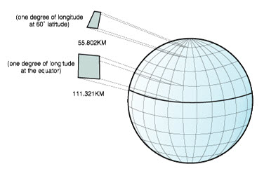
Fig. 22.6. Different dimensions between locations on the graticule.
(Source:http://publib.boulder.ibm.com/infocenter/db2luw/v9/index.jsp?topic=%2Fcom.ibm.db2.udb.spatial.doc%2Fcsb3022a.html; 3 December 2012)
A coordinate system can be defined by either a sphere or a spheroid approximation of the earth's shape. Because the earth is not perfectly round, a spheroid can help maintain accuracy for a map, depending on the location on the earth. A spheroid is an ellipsoid that is based on an ellipse, whereas a sphere is based on a circle.
The shape of the ellipse is determined by two radii. The longer radius is called the semimajor axis, and the shorter radius is called the semiminor axis. An ellipsoid is a three-dimensional shape formed by rotating an ellipse around one of its axes. Fig. 22.7 shows the sphere and spheroid approximations of the earth and the major and minor axes of an ellipse.
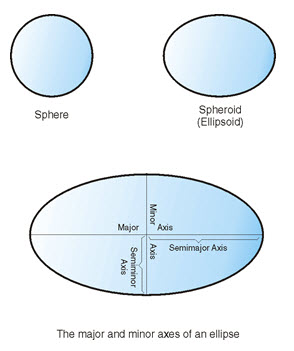
Fig. 22.7. Sphere and spheroid approximations.
(Source:http://publib.boulder.ibm.com/infocenter/db2luw/v9/index.jsp?topic=%2Fcom.ibm.db2.udb.spatial.doc%2Fcsb3022a.html; 3 December 2012)
22.2 Datum
A geodetic datum is a mathematical approximation of the Earth’s 3D surface and a reference from which other measurements are made. A datum is a set of values that defines the position of the spheroid relative to the center of the earth. The datum provides a frame of reference for measuring locations and defines the origin and orientation of latitude and longitude lines. Some datums are global and intend to provide good average accuracy around the world. A local datum aligns its spheroid to closely fit the earth's surface in a particular area. Therefore, the coordinate system's measurements are not be accurate if they are used with an area other than the one that they were designed. Fig. 22.8 shows how different datums align with the earth's surface. The local datum, NAD27, more closely aligns with Earth's surface than the Earth-centered datum, WGS84, at this particular location.
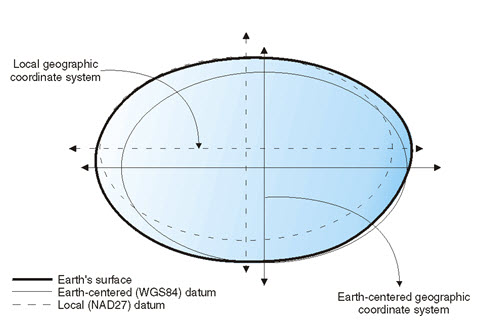
Fig. 22.8. Datum alignments.
(Source:http://publib.boulder.ibm.com/infocenter/db2luw/v9/index.jsp?topic=%2Fcom.ibm.db2.udb.spatial.doc%2Fcsb3022a.html; 3 December 2012)
Every spheroid has a major axis and a minor axis, with the major axis being the longer of the two but is not in itself a datum. The missing information is a description of how and where the shape deviates from the Earth’s actual surface. This is provided by the definition of a tie point, which is a known position on the Earth’s surface (or its interior, since the Earth’s centre of mass could be used), and its corresponding location on or within the ellipsoid.
Complications arise because datums may be global, regional or local, so that each is only accurate for a limited set of conditions. For a global datum, the tie point may well be the centre of mass of the Earth, meaning that the ellipsoid forms the best general approximation of the Earth’s shape, and that at any specific positions and accuracies may be quite poor. Such generalizations would be acceptable for datasets which are of very large or global extent. In contrast, a local datum, which uses a specific tie point somewhere on the surface, near the area of interest, would be used for a ‘local’ projector data set .Within this area, the deviation of the ellipsoid from the actual surface will be minimal but at some distance from it may be considerable. This is the reason behind the development of the great number of datums and projections worldwide. In practice, we choose a datum which is appropriate to our needs, according to the size and location of the area we are working with, to provide us with optimum measurement accurac. It is worth noting that in many cases there may be several different versions of datum and ellipsoid under the same name, depending on when, where, by whom and for which purpose they were developed. The differences between them may seem insignificant at first glance but, in terms of calculated ground distances, could produce very significant differences between measurements.
22.3 Geometric Distortions and Projection Models
Since paper maps and geospatial databases are flat representations of data located on a curved surface, the map projection is an accepted means for fitting all or part of that curved surface to the flat surface or plane. This projection cannot be made without distortion of shape, area, distance, direction or scale. We would ideally like to preserve all these characteristics but we cannot, so we must choose which of them should be represented accurately at the expense of others, or whether to compromise on several characteristics. Measuring exact distances from any map features in any direction would require constant scale throughout the map, but no map projection can achieve this. In most projections scale remains constant along one or more standard lines, and careful positioning of these lines can minimize scale variations elsewhere in the map. Specialized equidistant map projections maintain constant scale in all directions from one or two standard points. In many types of spatial analysis it is important to compare the areas of different features. Such comparisons require that surface features with equal areas are represented by the same map area regardless of where they occur. An equal-area map projection conserves area but distorts the shapes of features. A map projection is conformal if the shapes of small surface features are shown without distortion. This property is the result of correctly representing local angles around each point, and maintaining constant local scale in all directions. Conformality is a local property; while small features are shown correctly, large shapes must be distorted. A map projection cannot be both conformal and equal-area. No map projection can represent all great circle directions as straight lines. Azimuthal projections show all great circles passing through the projection center as straight lines. There are probably 20 or 30 different types of map projections in common usage. These have been constructed to preserve one or other characteristics of geometry, as follows:
1. Area: Many map projections try to preserve area, so that the projected region covers exactly the same area of the Earth’s surface no matter where it is placed on the map. To achieve this the map must distort scale, angles and shape.
2. Shape: There are two groups of projections which have either: (a) a conformal property where the angles and the shapes of small features are preserved, and the scales in x and y are always equal (although large shapes will be distorted); or (b) an equal area property where the areas measured on the map are always in the same proportion to the areas measured on the Earth’s surface but their shapes may be distorted.
3. Scale: No map projection shows scale correctly everywhere on the map, but for many projections there are one or more lines on the map where scale is correct.
4. Distance: Some projections preserve neither angular nor area relationships but distances in certain directions are preserved.
5. Angle: Although conformal projections preserve local angles, one class of projections (called azimuthal projections) preserve the easting an northing pair, so that angle and direction are preserved. Scale factor (k) is useful to quantify the amount of distortion caused by projection and is defined by the following:
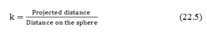
This relationship will be different at every point on the map and in many cases will be different in each direction. It only applies to short distances. The ideal scale factor is 1, which represents no distortion at all. Most scale factors approach but are less than 1.Any projection can achieve one or other of these properties but none can preserve all, and the distortions that occur in each case are illustrated schematically in Fig. 22.9. Once the property to be preserved has been decided, the next step is to transform the information using a ‘projectable’ or ‘flattenable’ surface. The transformation or projection is achieved using planar, cylindrical or cone-shaped surfaces that touch the Earth in one of a few ways; these form the basis for the three main groups of projection. Where the surface touches the Earth at a point (for a plane), along a great circle (for a cylinder) or at a parallel (for a cone), projections of the tangent type are formed. Where the surface cuts the earth, rather than just touching it, between two parallels, a secant type of projection is formed. The conic is actually a general form, with azimuthal and cylindrical forms being special cases of the conic type. In the planar type (such as a stereographic projection) where the surface is taken to be the tangent to one of the poles, the following relationship can be used to derive polar positions (all the equations given here assume a spherical Earth for simplicity):
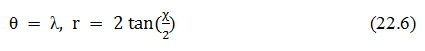
where x represents the colatitude ![]() the resultant polar coordinates can then be converted to planar coordinates using Equation (22.3). Of course, the plane could be a tangent to the Earth at any point, not just at one of the poles.
the resultant polar coordinates can then be converted to planar coordinates using Equation (22.3). Of course, the plane could be a tangent to the Earth at any point, not just at one of the poles.
For cylindrical projections, the axis of the cylinder may pass through the poles, for example, so that it touches the sphere at the equator (as in the Mercator). In this case, positions may be derived as:
For conic projections of the tangent type, the following can be used to derive positions, assuming one standard parallel at a colatitude of Χ0:
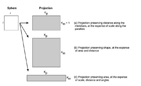
Fig. 22.9. Schematic illustration of the projection effects on a unit square of side length i, where K represents the scale along each projected side, and subscripts m and p represent meridian and parallel.
(Source: Jian & Philippa, 2009).

Fig. 22.10. Three main types of projections which are based on tangent case: planer (left), cylindrical (centre) and conical (right).
(Source: Jian & Philippa, 2009).
Keywords: Geographic coordinates, Datum, Projection, Equator, Spheroid. NAD27, WGS84.
References
Jian G. L. Philippa J. M. (2009) Essential image processing and GIS for Remote sensing, Wiley-Blackwell publications.
R. B. Smith (2011). Introduction to map projection, MicroImages, Inc., 1998-2011.
http://publib.boulder.ibm.com/infocenter/db2luw/v9/index.jsp?topic=%2Fcom.ibm.db2.udb.spatial.doc%2Fcsb3022a.html
http://www.microimages.com/documentation/Tutorials/project.pdf
Suggested Reading
http://ist.uwaterloo.ca/~abkirker/datums/index.html
http://www.microimages.com/documentation/Tutorials/project.pdf
http://en.wikipedia.org/wiki/Geographic_coordinate_system
http://geospatial.osu.edu/conference/proceedings/workshops/conner.pdf
http://www.ngi.gov.za/index.php/Geodesy-GPS/datums-and-coordinate-systems.html
http://webpages.marshall.edu/~jawolfe/lecture03.pdf
http://publib.boulder.ibm.com/infocenter/db2luw/v8/index.jsp?topic=/com.ibm.db2.udb.doc/opt/csb3022a.htm
http://www.tatamcgrawhill.com/html/9780070658981.html
Last modified: Friday, 31 January 2014, 7:47 AM