Remote Sensing & GIS Applications 3(2+1)

Lesson 26 Vector and Raster Map Algebra

26.1 Vector

With vector representation, the boundaries or the course of the features are defined by a series of points that, when joined with straight lines, form the graphic representation of that feature. The points themselves are encoded with a pair of numbers giving the X and Y coordinates in systems such as latitude/longitude or Universal Transverse Mercator grid coordinates. The attributes of features are then stored with a traditional database management (DBMS) software program. For example, a vector map of property parcels might be tied to an attribute database of information containing the address, owner's name, property valuation and land use. The link between these two data files can be a simple identifier number that is given to each feature in the map.

(Ronald, 1993)

26.2 Raster

The second major form of representation is known as raster. With raster systems, the graphic representation of features and the attributes they possess are merged into unified data files. In fact, they typically do not define features at all. Rather, the study area is subdivided into a fine mesh of grid cells in which the condition or attribute of the earth's surface at each cell point is recorded. Each cell is given a numeric value which may then represent a feature identifier, a qualitative attribute code or a quantitative attribute value.

For example, a cell could have the value "6" to indicate that it belongs to District 6 (a feature identifier), or that it is covered by soil type 6 (a qualitative attribute) or that it is 6 meters above sea level (a quantitative attribute value). Although the data we store in these grid cells do not necessarily refer to phenomena that can be seen in the environment, the data grids themselves can be thought of as images -- images of some aspect of the environment that can be made visible through the use of a raster display. In a raster display, such as the screen on your computer, there is also a grid of small cells called pixels. The term pixel is a contraction of picture element. Pixels can be made to vary in their colour, shape or grey tone. To make an image, the cell values in the data grid are used to regulate directly the graphic appearance of their corresponding pixels. Thus in a raster system, the data directly control the visible form we see. Vector and raster data can be represented as shown in Fig. 26.1. (Ronald, 1993).

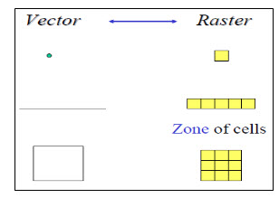
Fig. 26.1. Vector and Raster Data Representation. (Source: Ronald, 1993).

26.3 Raster versus Vector

Raster systems are typically data intensive (although good data compaction techniques exist) since they must record data at every cell location regardless of whether that cell holds information that is of interest or not. However, the advantage of the raster data structure is that geographical space is uniformly defined in a simple and predictable fashion. As a result, raster systems have substantially more analytical power than their vector counterparts in the analysis of continuous space and are thus ideally suited to the study of data that are continuously changing over space such as terrain, vegetation biomass, rainfall and the like. The second advantage of raster is that its structure closely matches the architecture of digital computers. As a result, raster systems tend to be very rapid in the evaluation of problems that involve various The basic data structure of vector systems can best be described as a network. As a result, it is not surprising to find that vector systems have excellent capabilities for the analysis of network space. Thus the difference between raster and vector is less one of inherent ability as it is of the difference in the types of space they describe. Mathematical combinations of the data in multiple grids. Hence they are excellent for evaluating environmental models such as those for soil erosion potential and forest management suitability. In addition, since satellite imagery employs a raster structure, most raster systems can easily incorporate these data and some provide full image processing capabilities. While raster systems are predominantly analysis oriented, vector systems tend to be more database management oriented.

Vector systems are quite efficient in their storage of map data because they only store the boundaries of features and not what is inside those boundaries. Because the graphic representation of features is directly linked to the attribute database, vector systems usually allow one to roam around the graphic display with a mouse and inquire about the attributes of any displayed feature: the distance between points or along lines, the areas of regions defined on the screen, and so on. In addition, they can produce simple thematic maps of database queries such as, "show all sewer line sections over one meter in diameter installed before 1940." (Ronald, 1993)

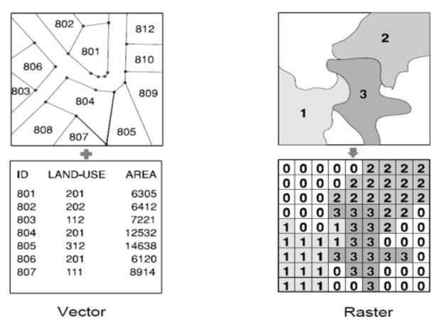
Fig. 26.2. Comparison between Vector and Raster data representation. (Source: Ronald, 1993)

Compared to their raster counterparts, vector systems do not have as extensive a range of capabilities for analysis over continuous space. However, they do excel at problems concerning movements over a network and can undertake the most fundamental of GIS operations. For many, it is the simple database management functions and excellent mapping capabilities that make vector systems attractive. Because of the close affinity between the logic of vector representation and traditional map production, a pen plotter can be driven to produce a map that is indistinguishable from that produced by traditional means. As a result, vector systems are very popular in municipal applications where issues of engineering map production and database management predominate. Raster and vector systems each have their special strengths. Some GIS incorporate elements from both representational techniques. Many systems provide most functions for one technique and provide limited display and data transfer functions using the other. Which technique is most appropriate depends upon the application. A complete GIS setup may include a vector system, a raster system, or both, depending upon the types of tasks that must be done. While some applications are suitable to either vector or raster, usually one is more appropriate. Using a system that is not well suited to a particular task can be very frustrating and lead to unsatisfactory results. (Ronald, 1993)

26.4 Raster Calculator

The Raster Calculator provides you a powerful tool for performing multiple tasks. You can perform mathematical calculations using operators and functions, set up selection queries, or type in Map Algebra syntax. Up to 4 rasters can be used in a single expression.  Inputs can be raster datasets or raster layers, coverage’s, shape files, tables, constants and numbers. The expressions are evaluated by the Raster Calculator on the fly and the user is provided with as status of the formula as he/she builds it. (http://www.ian-ko.com)

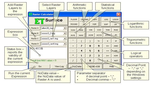
Fig. 26.3. Raster calculator showing expressions, functions and layers. (Source: http://www.ian-ko.com)

Inputs:

• Rasters - Up to 4 rasters can be used. If the Raster Calculator is used from the GUI, the rasters are selected from the raster layers loaded in Arc Map. In the Toolbox implementation the input can be a raster layer or raster dataset. The 4 rasters are called Raster A, Raster B, Raster C and Raster D. Raster A is required, the other rasters are optional.

• Expression - the formula to be used for the calculation to be performed. For shortness the rasters should be entered with their letters in the expression - A for Raster A, B for Raster B, etc. All the functions available can be typed in the expression box or selected from the calculator buttons provided. The functions are not case sensitive - SIN, Sin and sin will be accepted as correct entries. Note that the operator for EQUAL is "==" and NOT "=" (which is operator for assignment). The syntax of all functions is discussed below.

Output:

If the Raster Calculator is used from the GUI, the raster dataset created when an expression is executed is a temp raster and is stored in the temp folder of ET Surface. If you want to save it as a permanent raster, use the Export Data tool.

 If the Toolbox implementation is used, the user is asked for an output name and location and the raster dataset created is permanent.

(Source: http://www.ian-ko.com)

The output raster dataset will

• Be FLOAT type

• Have the cell size of the Raster A (if any of the other rasters used have a different cell size, it will be resampled).

• The extent will be calculated as the intersection of the extents of the input rasters.

(Source: http://www.ian-ko.com)

Functions performed by raster Calculator:

• The Raster Calculator tool allows for creating and executing a Map Algebra expression that will output a raster.

• Use the Layers and variables list to select the datasets and variables to use in the expression.

•  Numerical values and mathematical operators can be added to the expression by clicking the respective buttons in the tool dialog box. A list of commonly used conditional and mathematical tools is provided, allowing you to easily add them to the expression.

• Full paths to data or data existing in the specified current workspace environment setting can be entered in quotes (""). Numbers and scalars can be directly entered into an expression.

(http://help.arcgis.com)

Most conventional vector data models maintain data as multiple attribute maps, e.g. forest inventory polygons linked to a database table containing all attributes as columns. This basic distinction of raster data storage provides the foundation for quantitative analysis techniques. This is often referred to as raster or map algebra. (http://planet.botany.uwc.ac.za).

26.4.1 Map Algebra

This is in contrast to most conventional vector data models that maintain data as multiple attribute maps, e.g. forest inventory polygons linked to a database table containing all attributes as columns. This basic distinction of raster data storage provides the foundation for quantitative analysis techniques. This is often referred to as raster or map algebra. (http://planet.botany.uwc.ac.za).

Map algebra is a simple and an elegant set-based algebra for manipulating geographic data, proposed by Dr. Dana Tomlin in the early 1980s. It is a set of primitive operations in a geographic information system (GIS) which allows two or more raster layers ("maps") of similar dimensions to produce a new raster layer (map) using algebraic operations such as addition, subtraction etc. A set of tool that a GIS will typically provide is that for combining map layers mathematically. Modelling, in particular, requires that we be able to combine maps according to various mathematical combinations.

For example, we might have an equation that predicts mean annual temperature as a result of altitude. Or, as another example, consider the possibility of creating a soil erosion potential map based on factors of soil erosion, slope gradient and rainfall intensity. Clearly we need the ability to modify data values in our maps by various mathematical operations and transformations and to combine factors mathematically to produce the final result.

The Map Algebra tools will typically provide three different kinds of operations:

1. The ability to arithmetically modify the attribute data values over space by a constant (i.e., scalar arithmetic).

2. The ability to mathematically transform attribute data values by a standard operation (such as the trigonometric functions, log transformations and so on).

3. The ability to mathematically combine (such as add, subtract, multiply, divide) different data layers to produce a composite result.

This third operation is simply another form of overlay mathematical overlay, as opposed to the logical overlay of database query. To illustrate this, consider a model for snow melt in densely forested areas:

where M is the melt rate in cm/day, T is the air temperature and D is the dew point temperature. Given maps of the air temperatures and dew points for a region of this type, we could clearly produce a snow melt rate map. To do so would require multiplying the temperature map by 0.19 (a scalar operation), the dew point map by 0.17 (another scalar operation) and then using overlay to add the two results. This ability to treat maps as variables in algebraic formulas is an enormously powerful capability.

Map algebra provides one method to run spatial analyst tool. The Raster Calculator provides a powerful tool for performing multiple tasks. One can perform mathematical calculations using operators and functions, set up selection queries, or type in Map Algebra syntax. Inputs can be raster datasets or raster layers, coverages, shape files, tables, constants, and numbers. The set of operators is composed of arithmetical, relational, Boolean, bitwise, and logical operators that support both integer and floating-point values and combinatorial operators. (Ronald, 1993)

26.4.2 Raster data formats

Raster data models incorporate the use of a grid-cell data structure where the geographic area is divided into cells identified by row and column. This data structure is commonly called raster. While the term raster implies a regularly spaced grid other tessellated data structures do exist in grid based GIS systems. In particular, the quadtree data structure has found some acceptance as an alternative raster data model. (http://planet.botany.uwc.ac.za).

A raster data structure is in fact a matrix where any coordinate can be quickly calculated if the origin point is known, and the size of the grid cells is known. Since grid-cells can be handled as two-dimensional arrays in computer encoding many analytical operations are easy to program. This makes tessellated data structures a popular choice for many GIS software. Several tessellated data structures exist, however only two are commonly used in GIS's. The most popular cell structure is the regularly spaced matrix or raster structure. The use of raster data structures allow for sophisticated mathematical modelling processes while vector based systems are often constrained by the capabilities and language of a relational DBMS. (http://planet.botany.uwc.ac.za).

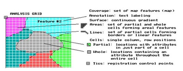
Fig. 26.4. Raster data formats. (Source: http://planet.botany.uwc.ac.za)

Since geographic data is rarely distinguished by regularly spaced shapes, cells must be classified as to the most common attribute for the cell. The problem of determining the proper resolution for a particular data layer can be a concern. If one selects too coarse a cell size then data may be overly generalized. If one selects too fine a cell size then too many cells may be created resulting in a large data volume, slower processing times, and a more cumbersome data set. As well, one can imply accuracy greater than that of the original data capture process and this may result in some erroneous results during analysis. So analysis mask. (http://planet.botany.uwc.ac.za).

Resampling or interpolation (and reprojection) of inputs to target extent, cell size, and projection within region defined by analysis mask.

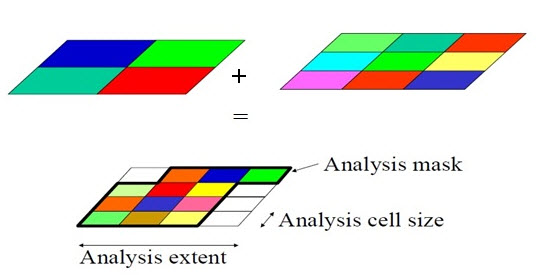
Fig. 26.5. Mask Analysis. (Source: Slides)

26.4.3 Vector-raster conversion

As well, since most data is captured in a vector format, e.g. digitizing, data must be converted to the raster data structure. This is called vector-raster conversion. Most GIS software allows the user to define the raster grid (cell) size for vector-raster conversion. It is imperative that the original scale, e.g. accuracy, of the data be known prior to conversion. The accuracy of the data, often referred to as the resolution, should determine the cell size of the output raster map during conversion. (http://planet.botany.uwc.ac.za).

26.4.3.1 Extracting information from surface

Some tools extract vector features from surfaces, or produce tabular summaries or smaller raster samples of surfaces. (http://planet.botany.uwc.ac.za).

Sampling rasters

The Sample tool creates a table that shows the values of a raster, or several rasters, at a set of sample point locations. The points can be in a point feature class or the cells in a raster that have values other than No Data. You might use this tool to get information about what occurs at a set of points, such as bird nesting sites, from terrain, distance to water, and forest type rasters.

(http://resources.arcgis.com).

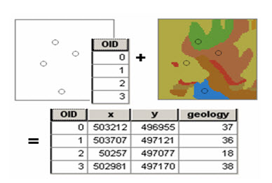
Fig. 26.6. Geology Raster Being Sampled at a set of points. (Source: http://resources.arcgis.com)

The output table can be analyzed on its own or joined to the sample point features. Below is an example of the sample results table joined back to the original sample points.

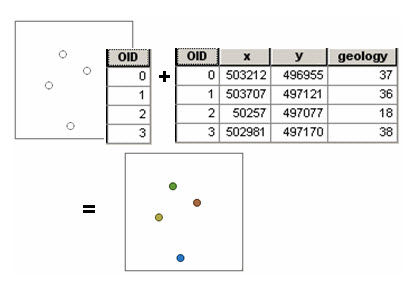
Fig. 26.7. Sample results Table joined back to the original sample points. (Source: http://resources.arcgis.com)

The Extract tools create a new raster with a copy of the cells within some mask area. The Extract By Mask tool lets you use a polygon feature class to extract the raster data.

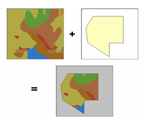
Fig. 26.8. New Raster which has been created. (http://resources.arcgis.com)

The Extract Values to Points tool creates a new feature class of points with the values of a single raster at a set of input point features. The Extract By Attributes tool selects cells of a raster based on a logical query. Extract By Polygon and Extract By Rectangle take lists of coordinate values that define an area and output a raster that is either inside or outside the polygon. Extract By Circle takes the centre coordinates and radius of a circle and outputs a raster that is either inside or outside the circle. Extract By Points takes a list of coordinate values that define a set of points and outputs a raster of the cell values at these points (or excluding these points). In all cases, the cells from the original raster that are not part of the Extract area are given No Data values. The 3D Analyst Surface Spot tool extracts elevation values from a surface for a set of point features and adds them to a Spot attribute of the points.

(http://resources.arcgis.com)

26.5 Application of Raster Calculator

In ArcGIS 10 the Spatial Analyst toolbox includes a Raster Calculator geoprocessing tool in the Map Algebra toolset.  This is not the same raster calculator as in previous versions of ArcGIS, so keep reading to find out what it does, how it’s improved, and where to find more information.

The Raster Calculator geoprocessing tool in ArcGIS 10 is designed to execute a single-line map algebra expression using multiple tools and operators listed on the tool dialog.  When multiple tools or operators from the tool dialog are used in one expression, the performance of this equation will generally be faster than executing each of the operators or tools individually. (http://blogs.esri.com)

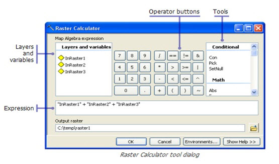
Fig. 26.9. Raster calculator Tool Dialog. (Source: http://blogs.esri.com) 

The Raster Calculator tool has been designed to replace both the previous Raster Calculator from the Spatial Analyst toolbar and the Single Output Map Algebra geoprocessing tool.  The Raster Calculator tool is like all other geoprocessing tools; it honors geoprocessing environment settings, it can be added to Model Builder, and when used in Model Builder it supports variables in the expression.  The ability to support variables in the expression makes the new Raster Calculator tool much more powerful and versatile than previous Map Algebra implementations.

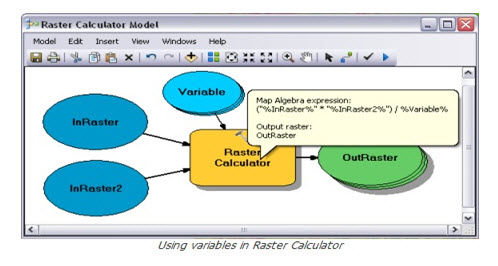
Fig. 26.10. Raster Calculator Model. (Source: http://blogs.esri.com)

The Raster Calculator tool is used to execute Map Algebra expressions inside ArcGIS applications.  The Raster Calculator is not supported in scripting because in ArcGIS 10 Map Algebra can be accessed directly when using the geoprocessing ArcPy site-package.  This seamless integration of Map Algebra into Python extends the capabilities of Map Algebra by taking advantage of Python and third party Python modules and libraries; making Map Algebra far more powerful than it has been in the past.  The Map Algebra language in ArcGIS 10 is similar to 9.x Map Algebra with minor syntax changes due to the integration of Python; most notably case sensitivity. (http://blogs.esri.com)

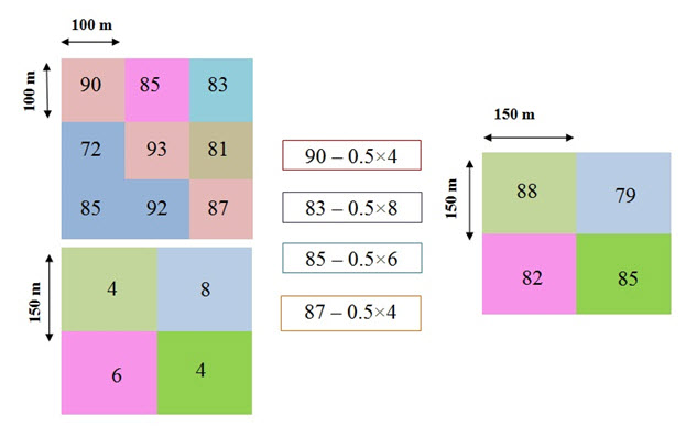
26.6 Raster Calculation Example

The grids below depict initial snow depth and average temperature over a day for an area.

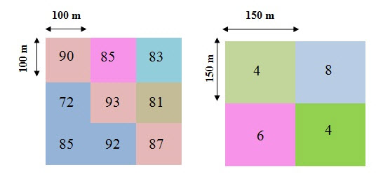
One way to calculate decrease in snow depth due to melt is to use a temperature index model that uses the formula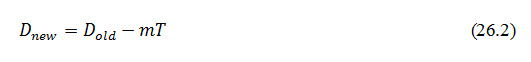

Here and  give the snow depth at the beginning and end of time step,T gives the temperature and m is melt factor m=0.5 cm/°C/day. Calculate the snow depth at the end of the day.

Solution:

Here using the [Eqn(26.2)] you can write

New depth at 100m = [Snow 100m]–0.5×[temp at 150m]             (26.3)

Converting the outputs to 150m grid:

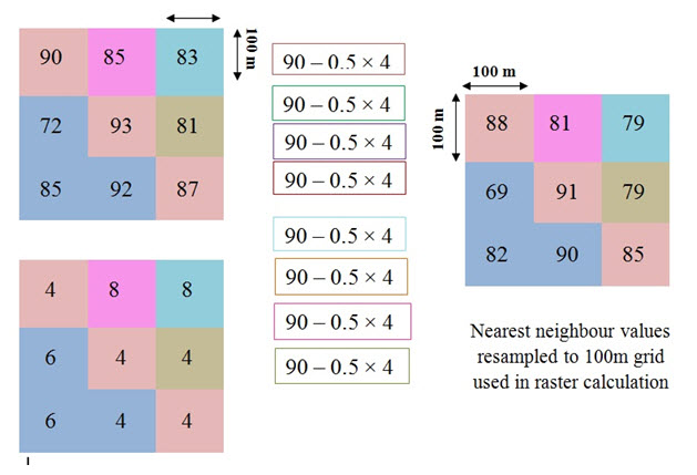
For conversion of 100m grid to 150m grid, it will follow the nearest neighbourhood rule.

First  you have to convert the 100m grid to 150m grid. Then you have to choose the nearest grid. And after choosing the nearest grid apply the above formula.

Converting temperature  to 100m grid:

For conversion follow the same nearest neighbour to the East and south for obtaining a 100 temperature grid.Then use  the Eqn (26.3).

26.7 Characteristics of Vector Data

There is no limit to the attribute information which can be stored or linked to a particular feature object. Tabular data represent a special form of vector data which can include almost any kind of data, whether or not they contain a geographic component; tabular data are not necessarily spatial in nature.

A table whose information includes and is referenced by coordinates can be displayed directly on a map. The information which does not must be linked to other spatial data that do have coordinates before it can be displayed on a map. Vector data therefore consist of a series of discrete features described by their coordinate positions than graphically or in any regularly structured way. The vector model could be thought of as the opposite of raster data in this respect, since it does not fill the space it occupies; not every conceivable location is represented, only those where some feature of interest exists.

If we were to choose the vector model to represent some phenomenon that varies continuously and regularly across a region, such that the vector data necessarily become so densely populated as to resemble a raster grid, then we would probably have chosen the wrong data model for those data. (Liu and Mason, 2009).

26.7.1 Buffers     

A zone calculated as the Euclidean distance from existing vector features, such as roads, is referred to as a buffer. Buffers are calculated at constant distance from the feature or at distances dictated by attribute values, and each zone will be the same width around the feature (see Fig. 26.11).

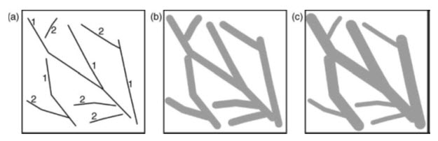
Fig. 26.11. (a) Simple vector line feature map, labelled with attribute values (1 and 2); (b) output with buffers of constant distance; (c) output map with buffers of distance defined by the attribute values shown in (a).

(Source: Liu and Mason, 2009).

Features with attribute value 1 having buffers twice the distance of those of features with attribute value 2. No-account is taken of the Earth’s curvature, so the zones will be at the same width regardless of the coordinate system. Negative distance values can be used, and these will cause a reduction in the size of the input feature. Buffers can also be generated on only one side of input features (should this be appropriate). The input layer in this case is a vector feature but the output may be a polygon file or raster. The same buffering operation can also be applied to raster data by first calculating the Euclidean distance and then reclassifying the output to exclude distances within or beyond specified thresholds; the output will always be a raster in this case. Buffering in this way can be considered as the vector equivalent of conditional logic combined with raster dilation or erosion. (Liu and Mason, 2009).

26.7.2 Dissolve

When boundaries exist between adjacent polygon or line features, they could be removed or dissolved because they have the same or similar values for a particular attribute (see Fig. 26.12). 

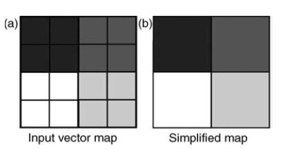
Fig. 26.12. Vector polygon features (a) and the Dissolved and simplified output map (b). (Source: Liu, and Mason, 2009)

As in a geological map where adjacent litho logical units with similar or identical descriptions can sensibly be joined into one, the boundaries between them are removed by this process and the classes merged intone. Complications in the vector case arise if the features’ attribute tables contain other attributes (besides the one of interest being merged) which differ across the boundary; choices must be made about how those other attributes should appear in the output dissolved layer. This is equivalent to merging raster classes through reclassification, or raster generalization/simplification. (Liu, and Mason, 2009).

26.7.3 Clipping

The geometry of a feature layer can be used as a mask to extract selectively a portion of another layer; the input layer is thereby clipped to the extent of the mask (see Fig. 26.13). The feature layer to be clipped may contain point, line or polygon features but the feature being used as a mask must have area, i.e. it will always be polygon.

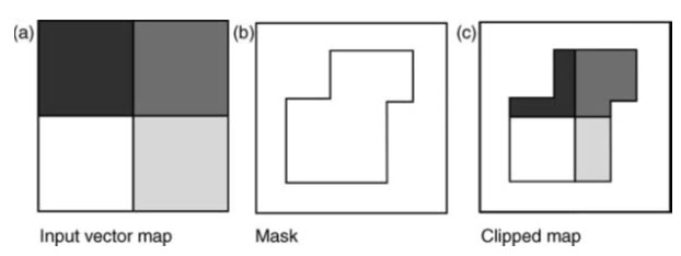
Fig. 26.13. Vector polygon clipping, using an input vector layer from which an area will be extracted (a), the vector feature whose geometric properties will be used as the mask (b) and (c) the vector output clipped feature. (Source: Liu and Mason, 2009)

The output feature attribute table will contain only the fields and values of the extracted portion of the input vector map, as the attributes of the mask layer are not combined. Clipping is equivalent to a binary raster zonal operation, where the pixels inside or outside the region are set as null, using a second layer to define the region or mask. (Liu and Mason, 2009).

26.7.4 Intersection

If two feature layers are to be integrated while preserving only those features that lie within the spatial extent of both layers, an intersection can be performed (see Figure 26.14).

This is similar to the operation except that the two input layers are not necessarily of the same feature type. The input layers could be point, line and/or polygon, so the output features could also be point, line and/or polygon in nature.

New vertices need to be created to produce the new output polygons, lines endpoints, through a process called cracking.

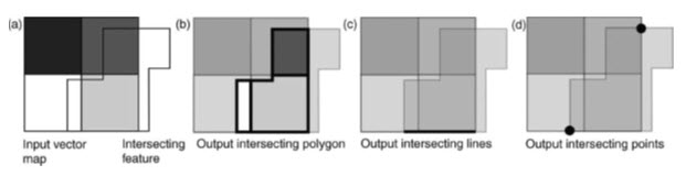
Fig. 26.14. Intersection operation between two overlapping polygon features (a); the output intersecting polygon (b) which covers the extent and geometry of the area which the two inputs have in common; the intersecting line (c) and points (d) shared by both polygons. The output attribute table contains only those fields and values that exist over the common area, line and points. (Source: Liu and Mason, 2009)

Unlike the clip operation, the output attribute table contains fields and values from both input layers, over the intersecting feature/area. In the case of two intersecting polygons, intersection is equivalent to a Boolean operation using a logical AND (Min) operator between two overlapping raster images.

When two input overlapping feature layers are required to be integrated such that the new output feature layer contains all the geometric features and attributes of two input layers, the union operation can be used (see Fig. 26.15).

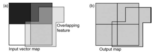
Fig. 26.15. Vector polygon union operation where two polygon features overlap (a) and the output object (b) covers the extent and geometry of both inputs. The output attribute table also contains the attribute fields and values of both input features. (Source: Liu and Mason, 2009)

Since vector feature layers can contain only points or only polygons, here the inputs must be of the same type but the number of inputs is not limited to two. Again, new vertices will be created through cracking. This is similar to the intersect operation but the output will have the total extent of the input layers. New, minor polygons are created wherever polygons overlap. The attribute table of the output layer contains attribute fields of both the input layers, though some of the entries may be blank. In the polygon case, it is equivalent to a binary raster operation using logical OR (Max) operator between overlapping images. (Liu and Mason, 2009).

Keywords: Raster Calculator, Map Algebra, Raster data formats, Sampling rasters, Buffers, Dissolve, Clipping, Intersection

Reference

• Ronald Eastman, J. Fulk., M and Toledano. J, 1993; The GIS Hand Book; Clark University; Washington.

• Liu, J.G, Mason P.J, 2009; Essential Image Processing and GIS For Remote Sensing; Imperial college, London, UK

• http://webhelp.esri.com

• http://help.arcgis.com

• http://blogs.esri.com

• http://www.ian-ko.com

• http://resources.arcgis.com

• http://planet.botany.uwc.ac.za

• Slides