Soil & Water Conservation Engg. 3(2+1)

Lesson 32 Case Study-Watershed Modelling for Soil and Water Conservation and Water Quality

32.1 Applications of Watershed Modelling

Watershed models help understand dynamic interactions between land surface hydrology and climate. For example, vegetation, snow cover and the permafrost active layer are some of the features which are quite sensitive to the lower boundary of the atmospheric system. The water and heat transfer between the land surface and atmosphere significantly influence hydrologic characteristics and yield, in turn, lower the boundary conditions for climate modelling.

Assessment of the impact of climate change on national water resources and agricultural productivity is made possible by the use of watershed models. Water allocation requires integration of watershed models with models of physical habitat, biological populations and economic response. Estimating the value of in-stream water use allows recreational, ecological and biological concerns to compete with traditional consumptive uses, such as agriculture, hydropower, municipality and industry. Watershed models are utilized to quantify the impacts of watershed management strategies linking human activities within the watershed to water quantity and quality of the receiving stream or lake for environmental and water resources protection.

32.2 Setting up a Watershed Model- Steps and Requirements

The modelling or model application, process can be described as comprised of three phases as shown in Fig. 32.1.  Phase I includes data collection, model input preparation and parameter evaluation, i.e. all the steps needed to set up a model, characterize the watershed and prepare for model executions.  Phase II is the model testing phase which involves calibration, validation and if possible a post-audit evaluation.  This is the phase in which the model is evaluated to assess whether it can reasonably represent the watershed behaviour for the purposes of the study.  Phase III includes the ultimate use of the model as a decision support tool for management and regulatory purposes.

Although specific application procedures for all watershed models differ due to the variations of the specific physical, chemical and biological systems each of them attempts to represent, they have many steps in common.  The calibration and validation phase is especially critical since the outcome establishes how well the model represents the watershed for the purpose of the study.  Thus, this is the ‘bottom-line’ of the model application effort as it determines if the model results can be relied upon and used effectively for decision-making.

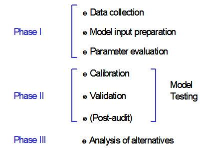
Fig. 32.1. Modelling Process. (Source: Singh and Frevert, 2002)

The data requirement for watershed modeling can be listed as:

1. Hydro-meteorologic, geo-morphologic, geologic, hydraulic and hydrologic (rainfall, snow, temperature, solar radiation, relative humidity, wind velocity and evapotranspiration)

2. Vegetation type, land use

3. Soil type, texture, infiltration, conductivity

4. Aquifer formation, rock type

5. Topography, slopes, length, area, perimeter (geo-morphometric)

6. Roughness, flow level, channel cross sections (hydraulic)

7. Flow depth, discharge, base flow, sub-surface flow (hydrologic)

32.3 Case Study

Watershed Modelling

A case study on water quantity, sediment yield and water quality is presented to analyse the scope of the hydrological model in particular SWAT (Soil Water and Assessment Tool) model. The model is a physically based, continuous time model, and simulates surface runoff, evapotranspiration, infiltration, percolation losses, channel transmission losses, channel routing, lateral flow as well as shallow and deep aquifer flow. It allows the partitioning of a watershed into a number of sub-watersheds and the input information for each sub-watershed is needed for modelling.

Study Area

The study was performed on Banha watershed with an area of 1,695 ha, located in the Upper Damodar Valley (UDV) in the Hazaribagh Command, District Chatra in Jharkhand, India (Fig. 32.2). The average annual rainfall in the area is 1200 mm of which more than 80% occurs during monsoon months from June to October and the rest in winter months (December and January). Daily temperature ranges from a maximum of 42.5°C (1st May, 1999) to a minimum of 2.5°C (18th January, 1999). Soils in the watershed are more or less uniform up to a depth of 0.5 m and vary texturally from loamy sand to loam with sandy loam as the common texture.

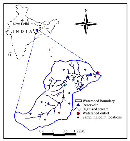
Fig. 32.2. Banha Watershed of DVC Command, Hazaribagh, Jharkhand, India. (Source: Mishra et al., 2007)

The land use/land cover of the area during rainy season mainly comprises rice crop, although black gram, maize, soybean and vegetables are also grown on some upland patches. The watershed has a mixed forest comprising sal (Shorea robusta), mahua (Madhuca indica), kend (Diospyros melanoxylon) and palas (Butea frondosa) trees in an area of about 878 ha (Fig. 32.3). In the area there is no source of factory effluent or point sources of water pollution. There is only rural effluent from individual houses. Chemical fertilizers and farm yard manures (FYM) are generally used in crop cultivation practices. Therefore, the sources of possible water quality/pollution (Non-Point Source) in the area are fertilizers, individual housing effluent and forest residues.

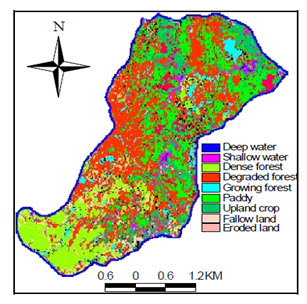
Fig. 32.3. Land Use/Land Cover Map of Banha Watershed for the Year 2000.

( Source: Mishra et al., 2007)

SWAT Model Description

In SWAT model, the surface runoff volume is estimated as shown below from daily rainfall by using the SCS curve number technique in which runoff is strongly influenced by the land cover/land use, soil type, slope and initial soil water content. The method reflects the effect of these factors on runoff generation from different areas of the watershed.

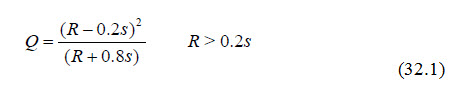
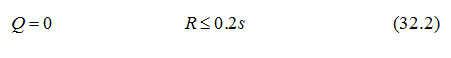
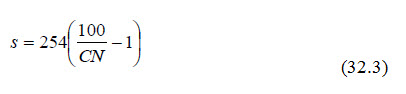
where, Q is the daily surface runoff (mm), R is the daily rainfall (mm) and s is a retention parameter (mm) which is related to the Curve Number (CN) and given as:

The sediment yield from each sub-basin of the watershed is computed by using the Modified Universal Soil Loss Equation (MUSLE). MUSLE uses the amount of runoff to simulate erosion and sediment yield.

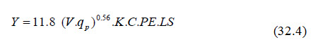
where Y is the sediment yield from the sub-basin at time t, V is the surface runoff volume for sub-basin in m³, q_p is the peak flow rate for sub-basin in m³/s, K is the soil erodibility factor, C is the crop management factor, PE is the erosion control practice factor and LS is the slope length and steepness factor. MUSLE uses the amount of runoff to simulate erosion and sediment yield.

For water quality assessment, SWAT uses the modified Erosion Productivity Impact Calculator (EPIC) model to compute nutrient yield and cycling from the sub-watersheds. In the present example (SWAT model application), the estimation of Nitrate-N and Phosphorous movement from the sub-watersheds along with the surface and sub-surface water is discussed briefly as given below.

Nitrate

The amount of NO₃-N contained in runoff, lateral flow and percolation are estimated as the product of the volume of water and concentration. The amount of NO₃-N in runoff is estimated for each sub-watershed by considering the top 10 mm soil layer only and is given as

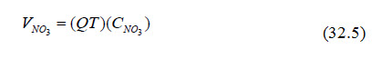
Where V_NO3 is the amount NO₃-N lost from the first layer, QT is the total water lost from the first layer in mm, and C_NO3 is the concentration of NO₃-N in the first layer. Leaching and lateral subsurface flows in lower layers are estimated with the same approach used in the upper layer, except that surface runoff is not considered. The loading function estimates the daily organic N runoff loss based on the concentration of organic N in the top soil layer, the sediment yield and enrichment ratio as

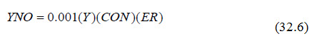
Where YNO is the organic N runoff loss at the outlet (kg/ha), CON is the concentration of organic N in the top soil layer (g/t), Y is the sediment yield (t/ha), and ER is the enrichment ratio and given as

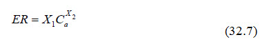
Where C_a is the sediment concentration (g/m³), and X₁ and X₂ are parameters set by the upper and lower limits. When the enrichment ratio approaches 1.0, the sediment concentration would be extremely high and will decrease with the reduction of ER.

Phosphorous

P is mostly associated with sediment and soluble P runoff in SWAT is expressed as

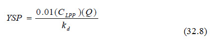
Where YSP is the soluble P (kg/ha) lost in runoff volume Q (mm), C_LPP is the concentration of soluble P in the soil layer (g/t), and k_d is the P concentration in the sediment divided by that of the water (m³/t). C_LPP is constant for the whole simulation and initially input to the model. The sediment-associated P is simulated with a loading function as

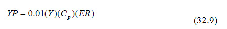
Where YP is the sediment associated P loss in runoff (kg/ha), C_p is the concentration of P in the top soil layer (g/t) and ER is the enrichment ratio.

The model performs simultaneous computation on each sub-watershed and routes water, sediment and nutrients through reaches and finally sums as loadings from the watershed.

Model Calibration

Calibration of the SWAT model was done using the measured data for the monsoon months of June to September of 2000. The time series of measured and model simulated daily stream flow and sediment yield from the watershed were compared, as shown in Figures 32.4 and 32.5 respectively.

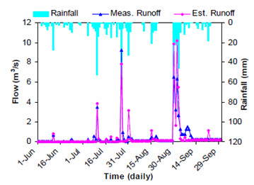
Fig. 32.4. Measured and SWAT Simulated Daily Flow.

(Source: Mishra et al., 2007)

The magnitude and temporal variation of simulated runoff showed a good response to rainfall distribution and a close match with the measured values, except that a few peaks marginally deviated from the measured daily runoff peaks. The differences between the measured and simulated runoff values can be ascribed to topographic and morphological heterogeneity of the watershed affecting the watershed runoff response.

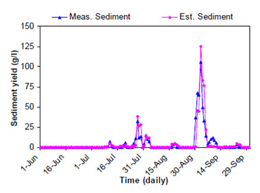
Fig. 32.5. Measured and SWAT Simulated Daily Sediment Yield.

(Source: Mishra et al., 2007)

The model simulated daily sediment yields were a little higher than the measured values for high rainfall events but for medium rainfall events the simulated values deviated less from the measured sediment yield. This can be attributed to the model rather than the rainfall characteristics. The differences can also be ascribed to the nature of rains and soil conditions over the watershed.

Simulation for Runoff and Sediment Yield

Using the measured rainfall and runoff data, the runoff response of the watershed was analyzed for the years 2000 and 2001 (Fig. 32.6). From the figure a close match between the rainfall and runoff is obtained which can be attributed to the small size of the watershed. For daily rainfall of less than 10 mm generated runoff is negligible particularly in the initial period of monsoon when the soil is relatively dry. Similarly for rainfall events at the end of monsoon, generated runoff was small due to less intense and intermittent rainfall events. Mid monsoon season runoff in July and August is distinctly higher for medium to high rainfall events due to sufficient soil wetness. In 2000 and 2001, the average daily rainfall was 6.0 and 5.0 mm with a standard deviation of 13.4 and 13.7 mm and the generated average daily runoff was 2.4 and 2.3 mm with a standard deviation of 6.3 and 3.7 mm, respectively. Monthly rainfall-runoff observations showed that proportion of runoff to rainfall was less initially but increased gradually towards the end of monsoon season. The trends of monthly runoff and rainfall were, however, exceptionally different in 2001 when the maximum values of rainfall and runoff occurred in the month of June and their magnitudes decreased successively in the remaining months (July–September) of the monsoon season.

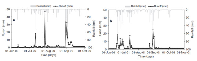
Fig. 32.6. Daily Rainfall/Runoff Distributions for the Years 2000 and 2001.

(Source: Mishra et al., 2007)

Regression analysis was performed to investigate the relationships among daily rainfall, runoff and sediment yield (Fig. 32.7 and 32.8). Slightly better correlation between rainfall and runoff with coefficients of determination of 0.83 and 0.76 in 2000 and 2001 respectively (Fig. 32.7) was found as against the respective values of 0.80 and 0.77 between rainfall and sediment yield (Fig. 32.8). It was also observed that a relatively uniform rainfall during the monsoon months in 2000 resulted in a better relationship compared to the year 2001 when rainfall was more non-uniformly distributed with time. Regression analyses revealed that daily rainfall had a higher influence on daily runoff and sediment yield, even though the watershed was multi-vegetated. The effect of land use and land cover (LULC) on sediment yield from different sub-watersheds was more conspicuous. Better forest cover and hence better protection of soil from the erosive effect of rains and overland flow resulted in smaller sediment yield. Higher infiltration of water in sub-watersheds with more area under forest cover prevented overland flow in rills and gullies and resulted in much less soil erosion rates. On the contrary, infiltration rate was lower in cultivated land and as a result runoff and sediment yield were higher.

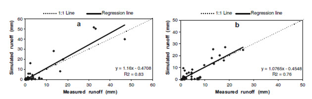
Fig. 32.7. Comparison between the Measured and SWAT Simulated Daily Runoff During June–September, 2000 (a) and June–October, 2001 (b).

(Source: Mishra et al., 2007)

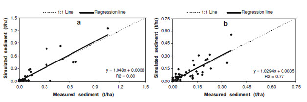
Fig. 32.8. Comparison between the Measured and SWAT Simulated Daily Sediment Yield During June–September, 2000 (a) and June–October, 2001 (b). (Source: Mishra et al., 2007)

Simulation for NPS Pollution

The calibrated SWAT model was used to simulate the water pollutants commonly known as Non-Point Source (NPS) pollution due to losses of nutrients from the watershed during June to September, 2000 and simulate the same during monsoon months of June to October of 2001. Measured concentrations of NO₃-N, NH₄-N and soluble P in the surface runoff at the watershed outlet in 2000 and 2001 were used for the validation of model simulations. Measured and simulated NO₃-N, NH₄-N and soluble P concentrations at the watershed outlet for both the seasons are presented in Fig. 32.9, 32.10 and 32.11 respectively.

From Fig. 32.9 it is seen that NPS NO₃-N loading for the year 2000 is generally closely predicted for all the events, with high statistical agreement, except for the initial events. Nash-Sutcliffe Efficiency coefficients values (0.95 and 0.99) and coefficient of determination values (0.99 and 0.99) indicate a high agreement for both the years.

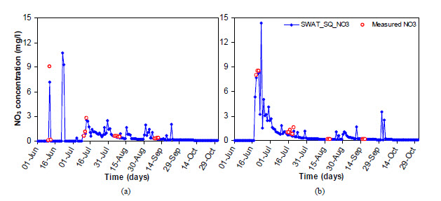
Fig. 32.9. Measured and SWAT Simulated NPS NO₃-N concentration at the Watershed Outlet in 2000 (a) and in 2001 (b). (Source: Mishra et al., 2009)

Comparison of the measured and simulated concentrations of NH₄-N for 2000 and 2001 shown in Fig. 32.10 a & b respectively reveal that the simulated values of NH₄-N are in close agreement with the measured values as indicated by the values of coefficients of determination (0.99 and 0.90) and Nash-Sutcliffe Efficiency coefficients (0.98 and 0.88). Statistical tests reveal that model predictions of NH₄-N are acceptable and may be used for the analysis of watershed behaviour.

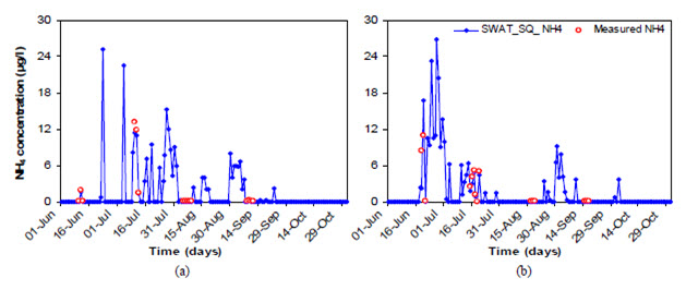
Fig. 32.10. Measured and SWAT Simulated NPS-NH₄-N concentration at the Watershed Outlet in 2000 (a) and in 2001 (b). (Source: Mishra et al., 2009)

Comparison between the measured and simulated values of soluble P for the selected observation dates of 2000 and 2001 (Fig. 32.11 a & b) reveal that the simulated values of soluble P are marginally under-predicted by the model. The values of coefficient of determination (0.98 for 2000 and 0.90 for 2001) and Nash-Sutcliffe simulation efficiencies (0.89 for 2000 and 0.83 for 2001) indicate a better agreement between the measured and simulated values for 2000. Overall statistical comparison shows that the model performance was satisfactory with respect to the simulation of soluble P.

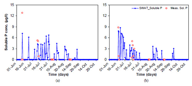
Fig. 32.11. Measured and SWAT Simulated NPS Water Soluble P  concentration at the Watershed Outlet in 2000 (a) and in 2001 (b).

(Source: Mishra et al., 2009)

Monthly surface and sub-surface losses of NO₃-N, NH₄- N, soluble P, organic N and organic P per unit area as NPS pollutants loads from the watershed to the downstream water were estimated from the validated SWAT model. The results obtained are shown in Figure 32.12. It is apparent that an appreciable amount of NO₃-N was lost in surface runoff with the percolated water. However, nutrient losses due to the sub-surface flow were relatively low. The loss of organic N was also quite high compared to organic P and NH₄-N. The quantified nutrient loads from the watershed varied from 2.57 to 4.52 kg/ha as NO₃-N lost in surface runoff, 0.17 to 0.29 kg/ha as NO₃-N lost in sub-surface runoff, 1.73 to 3.87 kg/ha as NO₃-N lost with percolated water, 0.13 to 0.14 kg/ha as organic-N, 0.02 kg/ha as NH₄-N, 0.02 kg/ha as organic P and 0.01 kg/ha as soluble P from the watershed as NPS pollutants during the monsoon months of 2000 and 2001. A clear variation in simulated losses of N and P for 2000 and 2001 is seen which is due to the variation in rainfall intensity and distribution in these two years and had a high effect on transport characteristics of NPS pollutants.

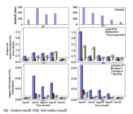
Fig. 32.12. SWAT Simulated Surface and Sub-surface Losses of NO₃-N, NH₄-N, Soluble P, Organic N and Organic P from the Watershed in 2000 and 2001. ( Source: Mishra et al., 2009)

32.4 Hydrological Modelling for Future Water Quantity Assessment

Climate variability and change are expected to alter regional hydrologic conditions and result in variety of impacts on water resource systems throughout the world. Potential impacts may include changes in hydrological processes such as evapotranspiration, soil moisture, water temperature, stream flow volume, timing and magnitude of runoff and frequency and severity of floods, all of which would cause changes in other environmental variables affecting plant growth.  Understanding the possible impacts of climate change on streamflow is of great importance for the appropriate design and management of water resources in any region. The effect of climate change on future water balance components at different sub-basins of the Krishna river basin is evaluated as an example. In order to accomplish this objective, SWAT (Soil and Water Assessment Tool), a distributed hydrologic model has been used. The future projected precipitation and temperature changes projected by PRECIS regional climate model under A1B emissions scenario were input into SWAT to predict the future streamflow changes. The results obtained from this example are expected to provide more insight into the availability of future streamflow and to provide local water management authorities with a planning tool.

Study Area: The Krishna river is the chosen area for this example. The Krishna River Basin (258,948 km²) located in semi-arid southern India is the fourth largest in India in terms of annual discharge, and fifth in terms of surface area. The drainage area of the entire basin is about 2,58,948 km² of which 26.8% lies in Maharashtra, 43.8% in Karnataka and 29.4 % in Andhra  Pradesh and its tributaries form an important integrated drainage system in the central portion of the Indian Peninsula. A major part of the water available in the Krishna basin originates from the humid regions of the Western Ghat mountains where precipitation exceeds 5000 mm. The river terminates at the Krishna delta in the Bay of Bengal.

Data inputs for Hydrological Modeling: The SWAT model requires data on terrain, land use, soil weather for the assessment of water-resources availability at desired locations of the drainage basin. To create a SWAT dataset, the interface needs to access ARC GIS with spatial analyst extension and data set files, which provide certain types of information about the watershed.

Spatial Data:

1. Digital Elevation Model (DEM)

2. Soil Data Layer

3. Land Use/ Land Cover layer

Climatic Data:  The model requires climatic data on

1. Precipitation

2. Maximum and minimum temperatures

3. Solar radiation

4. Wind speed

5. Relative humidity

For weather generator data set, observed climatology of the basin has been used.

Weather Data (Climate Model Data): The data generated in transient experiments PRECIS at a resolution 0.44° x 0.44° latitude by longitude RCM grid points was used for this study. The daily weather data on temperature (maximum and minimum), rainfall, solar radiation, wind speed and relative humidity at all the grid locations were processed. The centroid of each grid point was then taken as the location of weather station to be used in the SWAT model. This model has been used for processing the control/present (representing series (1960-1990) and the GHG (Green House Gas) A1B scenarios, (representing series 2011-2040 and 2041-2070).

Hydrological Modeling of the Basin: The Arc SWAT distributed hydrologic model has been used in this example.  The basin has been sub-divided into 23 sub-basins using the threshold value to divide the basin into a reasonable number of sub-basins so as to account for the spatial variability. After mapping the basin for terrain, land use and soil, simulated weather conditions predicted for control and GHG climate are incorporated into the model. The Krishna basin has been simulated using ARCSWAT model using generated daily weather data by PRECIS control climate scenario (1960-1990).  In this evaluation, the model has been used with the assumption that the river basin is a virgin area without any manmade changes. The model satisfactorily generates the detailed outputs on flow at sub-basin outflow points, actual evapotranspiration and soil moisture status at monthly intervals.

Changes in Water Balance Components: As mentioned above the monthly average precipitation, actual evapotranspiration, potential evapotranspiration, surface flow and water yield as simulated over the Krishna basin as a whole for control and two scenarios (A1B PRECIS, 2011 – 2040 and 2041 – 2070) have been obtained.  The variation in mean monthly water balance components from control to GHG scenario, both in terms of change in individual values of these components as well as percentage of change over control is shown in Fig. 32.13.

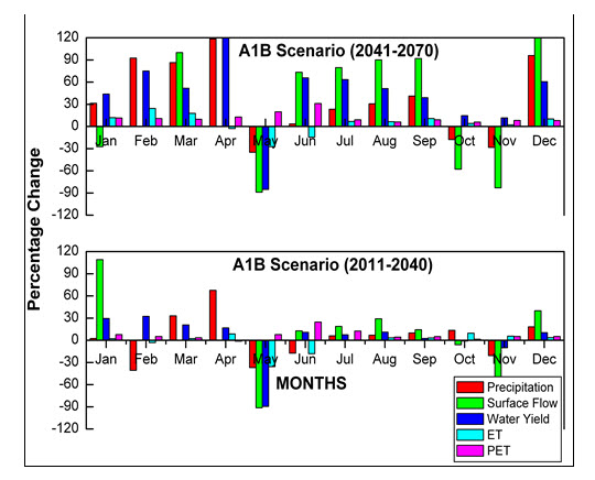
Fig. 32.13. Difference in Mean Monthly Water Balance Components from Control to GHG Scenario. (Source: Kulkanri and Bansod, 2012)

It may be observed from the above figures that increase in precipitation has been predicted in almost more than half of the months of the year, while decrease in precipitation for the remaining months has been predicted.  The magnitude of this increase/decrease in precipitation over the Krishna basin has been variable over various months.  The monthly average precipitation, actual evapotranspiration and water yield as simulated by the model over the basin will be increased during the period from 2041 to 2070.  

Limitations of the Method: It also should be noted that future flow conditions cannot be projected exactly due to uncertainty in climate change scenarios and GCM outputs. However, the general results of this analysis should be considered and incorporated into water resources management plans in order to promote more sustainable water use in the study area. In the assessment of impact of climate change on water availability, two models based on simplified assumptions were considered in the analyses and outputs. Hence, it is quite likely that the uncertainties presented in each of the models and the model outputs keep on accumulating while progressing towards the final output. These uncertainties include uncertainty linked to data quality, general circulation model (GCMs) and emission scenarios. The model simulations considered only future climate change scenarios assuming all other things as constants. But change in land use scenarios, soil, management activities and other climate variables will also contribute to some extent on water availability and crop production.

Conclusions: In this study projections of precipitation and evaporation change and their impacts on stream flow were investigated in the Krishna river basin for the 21^st century. The SWAT model is able to simulate the hydrology of the Krishna river basin successfully. The future annual discharge, surface runoff and baseflow in the basin show increases over the present as a result of future climate change. It should also be noted that future flow conditions cannot be projected exactly due to uncertainty in climate change scenarios and GCM outputs. However, the general results of this analysis should be identified and incorporated into water resources management plans in order to promote more sustainable water use in the study area. The major limitation of this study is that the model simulations considered only future climate change scenarios assuming all other things as constants. But change in land use scenarios, soil, management activities and other climate variables will also contribute greatly on water availability and crop production.

Keywords: Watershed Modelling, Soil and Water Conservation, Water Quality, Water Quantity, Sediment Yield.

References

Kulkarni B.D., Bansod S.D. (2012). Assessing hydrological response to changing climate in the Krishna basin. International confernece on Opportunities and challenges in monsoon prediction in a changing climate. Pune, India

Mishra, A., Kar, S. & Raghuwanshi, N.S. (2009) Modeling nonpoint source pollutant losses from a small watershed using HSPF model. Journal of Environmental Engineering, 2, 92-100

Mishra, A., Kar, S., Singh, V.P. (2007) Prioritizing structural management by quantifying the effect of land use and land cover on watershed runoff and sediment yield, Water Resources Management 21, 1899-1913.

Singh, V. P., & Frevert, D. K. (Eds.). (2002). Mathematical models of small watershed hydrology and applications. Water Resources Publication.

Suggested Readings

Manivanan, R. (2008) Water Quality Modeling: Rivers, Streams, and Estuaries. New Delhi, India: New India Publishing.

Owens, P. N., & Collins, A. J. (Eds.). (2006). Soil erosion and sediment redistribution in river catchments: measurement, modelling and management. CABI.